- Introduction
- Analytic Posteriors
- Posterior Estimation
- Forward-filtering Backward-sampling
- Non-Gaussian Extension
- Augmented FFBS Sampler
- Discussion
In this document we detail how dynamic linear models (DLMs) can be implemented in Theano (or similar tensor libraries), as well as a complementary Rao-Blackwellized sampler tailored to the structure of DLMs. Furthermore, we provide an example of how DLMs can be extended–via Gaussian scale-mixtures–to model non-gaussian observations. The example is a Pólya-Gamma extension to forward-filtering backward-sampling for negative-binomial observations.
Introduction
For a proper introduction of dynamic linear models and their estimation, see Harrison & West (1999),Petris, Petrone & Campagnoli (2009), and Gamerman & Lopes (2006),Pole, West & Harrison (1994). The focus of this document is on some practical details behind DLM estimation in Python–and, particularly, libraries like Theano (Bergstra, Breuleux, Bastien, Lamblin, Pascanu, Desjardins, Turian, Warde-Farley & Bengio 2010). Throughout, we use some custom random variable objects from symbolic-pymc (Willard 2019). This is largely because symbolic-pymc offers a necessary non-standard distribution and its random variables work well within the scan operations we employ.
In the future, we plan to build optimizations that automate much of the work done here (and more). This exposition sets the foundation for such work by first motivating the use and generality of Bayesian frameworks like DLMs, then by demonstrating the analytic steps that produce customized, efficient samplers. These are the steps that would undergo automation in the future.
A DLM with prior \(\theta_0 \sim \operatorname{N}\left( m_0, C_0 \right)\) is defined as follows:
\[\begin{align} y_t &= F_t^{\top} \theta_{t} + \epsilon_t, \quad \epsilon_t \sim \operatorname{N}\left( 0, V_t \right) \label{eq:basic-dlm-obs} \\ \theta_t &= G_t \theta_{t-1} + \nu_t, \quad \nu_t \sim \operatorname{N}\left( 0, W_t \right) \label{eq:basic-dlm-state} \end{align}\]
for \(t \in \{1, \dots, T\}\), \(y_t \in \mathbb{R}\), and \(\theta_t \in \mathbb{R}^{M}\).
The most “notationally” faithful representation of the timeseries model in \(\eqref{eq:basic-dlm-state}\) using Theano is provided in Listing 2. It represents the notion of a recursion–to the best of Theano’s ability–by way of the scan operator.
import numpy as np

import theano
import theano.tensor as tt

import matplotlib.pyplot as plt

from cycler import cycler

from matplotlib.collections import LineCollection

from theano.printing import debugprint as tt_dprint

from symbolic_pymc.theano.random_variables import NormalRV, MvNormalRV, GammaRV


plt.style.use('ggplot')
plt_orig_cycler = plt.rcParams['axes.prop_cycle']
plt.rc('text', usetex=True)

# theano.config.cxx = ""
# theano.config.mode = "FAST_COMPILE"
tt.config.compute_test_value = 'ignore'
N_obs_tt = tt.iscalar("N_obs")
N_theta_tt = tt.iscalar("N_theta")

G_tt = tt.specify_shape(tt.matrix(), [N_theta_tt, N_theta_tt])
G_tt.name = 'G_t'

F_tt = tt.specify_shape(tt.col(), [N_theta_tt, 1])
F_tt.name = 'F_t'

rng_state = np.random.RandomState(np.random.MT19937(np.random.SeedSequence(1234)))
rng_init_state = rng_state.get_state()
rng_tt = theano.shared(rng_state, name='rng', borrow=True)
rng_tt.tag.is_rng = True
rng_tt.default_update = rng_tt

m_0_tt = tt.zeros([N_theta_tt])
m_0_tt.name = "m_0"
C_0_tt = 1000.0 * tt.eye(N_theta_tt)
C_0_tt.name = "C_0"

theta_0_rv = MvNormalRV(m_0_tt, C_0_tt, rng=rng_tt, name='theta_0')

phi_W_true = np.r_[5.0, 10.0]
phi_W_tt = theano.shared(phi_W_true, name='phi_W')
W_tt = tt.eye(N_theta_tt) * tt.inv(phi_W_tt)
W_tt.name = "W_t"

phi_V_true = 0.1
phi_V_tt = theano.shared(phi_V_true, name='phi_V')
V_tt = tt.inv(phi_V_tt)
V_tt.name = "V_t"

def state_step(theta_tm1, G_t, W_t, N_theta, rng):
    nu_rv = MvNormalRV(tt.zeros([N_theta]), W_t, rng=rng, name='nu')
    theta_t = G_t.dot(theta_tm1) + nu_rv
    return theta_t


theta_t_rv, theta_t_updates = theano.scan(fn=state_step,
                                          outputs_info={"initial": theta_0_rv, "taps": [-1]},
                                          non_sequences=[G_tt, W_tt, N_theta_tt, rng_tt],
                                          n_steps=N_obs_tt,
                                          strict=True,
                                          name='theta_t')

def obs_step(theta_t, F_t, V_t, rng):
    eps_rv = NormalRV(0.0, tt.sqrt(V_t), rng=rng, name='eps')
    y_t = F_t.T.dot(theta_t) + eps_rv
    return y_t


Y_t_rv, Y_t_updates = theano.scan(fn=obs_step,
                                  sequences=[theta_t_rv],
                                  non_sequences=[F_tt, V_tt, rng_tt],
                                  strict=True,
name='Y_t')Throughout we’ll use data sampled from \(\eqref{eq:basic-dlm-state}\) for demonstration purposes. Our simulation has the following model parameter values:
\[\begin{equation} \begin{gathered} T = 200,\quad M = 2 \\ W_t = \operatorname{diag}\left( \phi_W \right) ,\quad V_t = \operatorname{diag}\left( \phi_V \right) \\ \phi_W = \left(1.1, 10\right),\quad \phi_V = 0.7 \\ G_t = \begin{pmatrix} 1 & 0.1 \\ 0 & 1 \\ \end{pmatrix},\quad F_t = \begin{pmatrix} 1 \\ 0 \end{pmatrix} \\ \theta_0 = \begin{pmatrix} 0 \\ 0 \end{pmatrix} \end{gathered} \label{eq:sim-settings} \end{equation}\]
A sample from \(\eqref{eq:sim-settings}\) is generated in Listing 3.
from theano import function as tt_function

dlm_sim_values = {
    N_obs_tt: 200,
    N_theta_tt: 2,
    G_tt: np.r_['0,2',
                [1.0, 0.1],
                [0.0, 1.0]].astype(tt.config.floatX),
    F_tt: np.r_[[[1.0],
                 [0.0]]].astype(tt.config.floatX)
}

rng_tt.get_value(borrow=True).set_state(rng_init_state)

simulate_dlm = tt_function([N_obs_tt, N_theta_tt, G_tt, F_tt],
                           [Y_t_rv, theta_t_rv],
                           givens={theta_0_rv: np.r_[0.0, 0.0]},
                           updates=Y_t_updates)

y_sim, theta_t_sim = simulate_dlm(dlm_sim_values[N_obs_tt], dlm_sim_values[N_theta_tt], dlm_sim_values[G_tt], dlm_sim_values[F_tt])

rng_sim_state = rng_tt.get_value(borrow=True).get_state()In Figure 4 we plot a sample from the model in Listing 2 for a fixed RNG seed.
plt.clf()

fig, ax = plt.subplots(figsize=(8, 4.8))
_ = ax.plot(y_sim, label=r'$y_t$', color='black', linewidth=0.7)

plt.tight_layout()
plt.legend()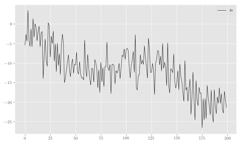
Analytic Posteriors
The standard DLM is essentially a Kalman Filter and enjoys many well documented closed-form results. In the following, we will simply state the relevant prior predictive and posterior results.
Given all the prior and observed data up to time \(t\), \(D_t\), these distribution are given by the following:
\[\begin{align} \theta_{t} \mid D_{t-1} &\sim \operatorname{N}\left( a_{t}, R_{t} \right) \\ y_{t} \mid D_{t-1} &\sim \operatorname{N}\left( f_{t}, Q_{t} \right) \end{align}\]
The prior predictive moments are as follows:
\[\begin{equation} \begin{gathered} a_t = G_t m_{t-1}, \quad R_t = G_t C_{t-1} G_t^\top + W_t \\ f_t = F_t^\top a_{t}, \quad Q_t = F_t^\top C_{t-1} F_t + V_t \end{gathered} \label{eq:dlm-prior-predictive} \end{equation}\]
We’ll also want to compute the posterior moments for \(\theta_t \mid D_t\), which are as follows:
\[\begin{equation} \begin{gathered} m_t = a_{t} + R_t F_t Q_t^{-1} \left(y_t - f_t\right), \quad C_t = R_t - R_t F_t Q_t^{-1} F_t^\top R_t \end{gathered} \label{eq:dlm-post-moments} \end{equation}\]
These “filtered” moments/distributions are one “kind” of posterior result for a DLM, and they only take into account the data up to time \(t\). The other kind are the “smoothed” distributions, which provide posterior distributions for each time \(t\) given all observations preceding and following \(t\).
Notationally, we’ve used \(D_t\) to signify all conditional observations and parameters up to time \(t\), so the smoothed distributions are given by \(\theta_t \mid D_T\), in contrast to \(\theta_t \mid D_t\)
The smoothed \(\theta_t\) distributions are still Gaussian, i.e. \(\left(\theta_t \mid D_T\right) \sim \operatorname{N}\left(s_t, S_t\right)\), and their moments are as follows:
\[\begin{equation} \begin{aligned} s_t &= m_t + C_t G_{t+1}^\top R_{t+1}^{-1} \left( s_{t+1} - a_{t+1} \right) \\ S_t &= C_t - C_t G_{t+1}^\top R_{t+1}^{-1} \left( R_{t+1} - S_{t+1} \right) R_{t+1}^{-1} G_{t+1} C_t \end{aligned} \label{eq:dlm-smooth-moments} \end{equation}\]
In most cases, models will not be as simple as the standard DLM. Even so, these basic closed-form solutions can still be relevant. For instance, efficient MCMC algorithms can be constructed using these closed-form results for conditionally linear models. In those cases, we can compute the posterior moments–in closed-form–conditional on samples generated by other means.
The standard approach is called forward-filtering backward-sampling (FFBS) and uses smoothed posteriors \(\theta_t \mid \theta_{t+1}, D_T\) conditioned on all other parameters.
We’ll build up to forward-backward sampling in what follows, but, first, we need to establish how the requisite quantities can be computed symbolically.
Posterior Estimation
In Listings 6 and 7, we demonstrate how the posterior moments in \(\eqref{eq:dlm-post-moments}\) and \(\eqref{eq:dlm-smooth-moments}\) can be computed in Theano.
Unfortunately, if we attempt to implement the exact closed-form updates in \(\eqref{eq:dlm-post-moments}\) or \(\eqref{eq:dlm-smooth-moments}\), our results will be fraught with numerical errors. This is a very basic issue with naively implemented Kalman filters. The solution to these issues usually involves some analytic reformulations that compensate for the covariance matrix subtractions. The standard approaches generally use some form of matrix decomposition that directly accounts for the positive semi-definite nature of the covariance matrices.
The approach taken here is based on the singular value decomposition (SVD) and effectively computes only one symmetric “half” of the updated covariances. The SVD also allows for easy inversions. See Zhang & Li (1996) for more details, or Petris, Petrone & Campagnoli (2009) for a concise overview of the procedure in the context of DLMs.
import warnings

warnings.filterwarnings("ignore", category=FutureWarning, message="Using a non-tuple sequence")

from theano.tensor.nlinalg import matrix_dot


def tt_finite_inv(x, eps_truncate=False):
    """Compute the element-wise reciprocal with special handling for small inputs.

    Parameters
    ==========
    x: Tensor-like
        The value for which the reciprocal, i.e. `1/x`, is computed.

    eps_truncate: bool (optional)
        Determines whether or not a floating-point epsilon truncation is used to
        upper-bound the returned values.
        If not (the default), infinite values are simply set to zero.
    """
    if eps_truncate:
        eps = np.finfo(getattr(x, 'dtype', None) or theano.config.floatX).eps
        return tt.minimum(tt.inv(x), np.reciprocal(np.sqrt(eps)))
    else:
        y = tt.inv(x)
        res_subtensor = y[tt.isinf(y)]
        return tt.set_subtensor(res_subtensor, 0.0)
SVD-based Filtering
The SVD forms of the filtering equations in \(\eqref{eq:dlm-post-moments}\) are produced through creative use of the SVDs of its component matrices. Using a slightly modified version of the formulation established in Petris, Petrone & Campagnoli (2009), the SVD for a matrix \(M\) is given by \(M = U_{M} D_{M} V_{M}^\top\). A symmetric matrix then takes the form \(M = U_{M} D_{M} U_{M}^\top\) and its “square-root” is given by \(M = N_M^\top N_M\) with \(N_M = S_{M} U_{M}^\top\) and \(S_{M} = D_{M}^{1/2}\). Likewise, matrix (generalized) inverses take the form \(M^{-1} = U_{M} S_{M}^{-1} U_{M}^\top\).
The idea here is that we can combine these SVD identities to derive square-root relationship between the SVD of \(C_t^{-1}\) and the SVDs of \(C_{t-1}\), \(W_t\), \(V_t\), and \(R_t\), then we can easily invert \(C_t^{-1}\) to arrive at the desired numerically stable SVD of \(C_t\).
First, note that \(N_{R_t}^\top N_{R_t} = G_t C_{t-1} G_t^\top + W_t = R_t\) for
\[\begin{equation} \begin{aligned} N_{R_t} &= \begin{pmatrix} S_{C_{t-1}} U_{C_{t-1}}^\top G_t^\top \\ N_{W_t} \end{pmatrix} \end{aligned} . \label{eq:N_R_t} \end{equation}\]
From this, we know that the SVD of \(R_t\) can be easily derived from the SVD of its square root, \(N_{R_t}\), i.e. \(U_{R_t} = V_{N_{R_t}}\) and \(S_{R_t} = D_{N_{R_t}}\). In other words, we can obtain a matrix’s SVD by computing the SVD of its “half”, which is itself entirely comprised of previous SVD components. The inherent symmetry of our covariance matrices is nicely preserved because we’re only ever using and computing one “half” of these matrices.
With the updated SVD of \(R_t\), we can use the identity \(C_t^{-1} = F_t V_t^{-1} F_t^\top + R_t^{-1}\)–obtained via the classic Sherman-Morrison-Woodbury matrix inverse identity–to employ the same technique as before and produce the SVD of \(C_t^{-1}\) by way of the SVD of yet another block square-root matrix,
\[\begin{equation} \begin{aligned} N_{C_t^{-1}} &= \begin{pmatrix} N_{V_t^{-1}} F_t^\top U_{R_t} \\ S_{R_t}^{-1} \end{pmatrix} \end{aligned} . \label{eq:N_C_t_inv} \end{equation}\]
Again, we compute the SVD of \(N_{C_t^{-1}}\) at this step and obtain \(V_{N_{C_t^{-1}}}\) and \(D_{N_{C_t^{-1}}}\).
This time, the block square-root matrix relationship isn’t so direct, and we have to multiply by \(U_{R_t}\): \(U_{R_t} N_{C_t^{-1}}^\top N_{C_t^{-1}} U_{R_t}^\top = C_t^{-1}\). However, since the additional \(U_{R_t}\) terms are orthogonal, we are able to derive the SVD of \(C_t\) as \(U_{C_t} = U_{R_t} V_{N_{C_t^{-1}}}\) and \(S_{C_t} = D_{N_{C_t^{-1}}}^{-1}\).
These quantities are computed in Listing 6.
from theano.tensor.nlinalg import svd


y_tt = tt.specify_shape(tt.col(), [N_obs_tt, 1])
y_tt.name = 'y_t'


def filtering_step(y_t, m_tm1, U_C_tm1, S_C_tm1, F_t, G_t, N_W_t, N_V_t_inv):
    """Compute the sequential posterior state and prior predictive parameters."""

    # R_t = N_R.T.dot(N_R)
    N_R = tt.join(0,
                  matrix_dot(S_C_tm1, U_C_tm1.T, G_t.T),
                  N_W_t)
    # TODO: All this could be much more efficient if we only computed *one* set of singular
    # vectors for these non-square matrices.
    _, d_N_R_t, V_N_R_t_T = svd(N_R)

    U_R_t = V_N_R_t_T.T
    S_R_t = tt.diag(d_N_R_t)
    S_R_t_inv = tt.diag(tt_finite_inv(d_N_R_t))

    N_C_t_inv = tt.join(0,
                        matrix_dot(N_V_t_inv, F_t.T, U_R_t),
                        S_R_t_inv)
    _, d_N_C_t_inv, V_N_C_t_inv_T = svd(N_C_t_inv)

    U_C_t = U_R_t.dot(V_N_C_t_inv_T.T)
    d_C_t = tt_finite_inv(tt.square(d_N_C_t_inv))
    D_C_t = tt.diag(d_C_t)
    S_C_t = tt.diag(tt.sqrt(d_C_t))

    C_t = matrix_dot(U_C_t, D_C_t, U_C_t.T)

    a_t = G_t.dot(m_tm1)
    f_t = F_t.T.dot(a_t)
    # A_t = R_t @ F_t @ inv(Q_t) = C_t @ F_t @ inv(V_t)
    m_t = a_t + matrix_dot(C_t, F_t, N_V_t_inv.T, N_V_t_inv, y_t - f_t)

    return [m_t, U_C_t, S_C_t, a_t, U_R_t, S_R_t]


_, d_C_0_tt, Vt_C_0_tt = svd(C_0_tt)
U_C_0_tt = Vt_C_0_tt.T
S_C_0_tt = tt.diag(tt.sqrt(d_C_0_tt))

_, d_W_tt, Vt_W_tt = svd(W_tt)
U_W_tt = Vt_W_tt.T
s_W_tt = tt.sqrt(d_W_tt)
N_W_tt = tt.diag(s_W_tt).dot(U_W_tt.T)

_, D_V_tt, Vt_V_tt = svd(tt.as_tensor_variable(V_tt, ndim=2) if V_tt.ndim < 2 else V_tt)
U_V_tt = Vt_V_tt.T
S_V_inv_tt = tt.diag(tt.sqrt(tt_finite_inv(D_V_tt, eps_truncate=True)))
N_V_inv_tt = S_V_inv_tt.dot(U_V_tt.T)


filter_res, filter_updates = theano.scan(fn=filtering_step,
                                         sequences=y_tt,
                                         outputs_info=[
                                             {"initial": m_0_tt, "taps": [-1]},
                                             {"initial": U_C_0_tt, "taps": [-1]},
                                             {"initial": S_C_0_tt, "taps": [-1]},
                                             {}, {}, {}, # a_t, U_R_t, S_R_t
                                         ],
                                         non_sequences=[F_tt, G_tt, N_W_tt, N_V_inv_tt],
                                         strict=True,
                                         name='theta_filtered')

(m_t, U_C_t, S_C_t, a_t, U_R_t, S_R_t) = filter_resSVD-based Smoothing
We can use the techniques above to produce SVD versions of the smoothing equations in \(\eqref{eq:dlm-smooth-moments}\). In this case, some extra steps are required in order to SVD-decompose \(S_t\) in the same manner as \(R_t\) and \(C_t^{-1}\) were.
First, notice that our target, \(S_t\), is a difference of matrices, unlike the matrix sums that comprised \(R_t\) and \(C_t^{-1}\) above. Furthermore, \(S_t\) is given as a difference of a (transformed) difference. To address the latter, we start by expanding \(S_t\) and setting \(B_t = C_t G_{t+1}^\top R_{t+1}^{-1}\) to obtain
\[\begin{equation} \begin{aligned} S_t &= C_t - B_t R_{t+1} B_t^\top + B_t S_{t+1} B_t^\top \\ &= H_t + B_t S_{t+1} B_t^\top \end{aligned} \label{eq:S_t_decomp} \end{equation}\]
Having turned \(S_t\) into a sum of two terms, we can now consider another blocked SVD-based square-root reformulation, which starts with the reformulation of \(H_t\).
We can use the definition of \(R_t = G_{t+1} C_t G_{t+1}^\top + W_{t+1}\) to get
\[\begin{equation} \begin{aligned} H_t &= C_t - B_t R_{t+1} B_t^\top \\ &= C_t - C_t G_{t+1}^\top R_{t+1}^{-1} G_{t+1} C_t \\ &= C_t - C_t G_{t+1}^\top \left(G_{t+1} C_t G_{t+1}^\top + W_{t+1}\right)^{-1} G_{t+1} C_t . \end{aligned} \end{equation}\]
This form of \(H_t\) fits the Woodbury identity and results in \(H_t^{-1} = G_{t+1}^\top W_{t+1}^{-1} G_{t+1} + C_t^{-1}\), which is amenable to our square-root formulation.
Specifically, \(H_t^{-1} = U_{C_t} N_{H_t}^{-\top} N_{H_t}^{-1} U_{C_t}^\top\), where
\[\begin{equation} \begin{aligned} N_{H_t}^{-1} &= \begin{pmatrix} N_{W_{t+1}}^{-1} G_{t+1} U_{C_t} \\ S_{C_t}^{-1} \end{pmatrix} \end{aligned} . \label{eq:N_H_t_inv} \end{equation}\]
By inverting the SVD of \(N_{H_t}^{-1}\) we obtain the SVD of \(H_t\) as \(U_{H_t} = U_{C_t} V_{N_{H_t}^{-1}}\) and \(D_{H_t} = {D_{N_{H_t}^{-1}}}^{-2} = S_{H_t}^2\).
Finally, using \(\eqref{eq:S_t_decomp}\) and \(\eqref{eq:N_H_t_inv}\) we can derive the last blocked square-root decomposition \(S_t = N_{S_t}^\top N_{S_t}\):
\[\begin{equation} \begin{aligned} N_{S_t} &= \begin{pmatrix} S_{H_t} U_{H_t}^\top \\ S_{S_{t+1}} U_{S_{t+1}}^\top B_t^\top \end{pmatrix} \end{aligned} . \label{eq:N_S_t} \end{equation}\]
Again, we take the SVD of \(N_{S_t}\) and derive the SVD of \(S_t\) as \(U_{S_t} = V_{N_{S_t}}\) and \(D_{S_t} = D_{N_{S_t}}^2 = S_{S_t}^2\).
def smoother_step(m_t, U_C_t, S_C_t, a_tp1, U_R_tp1, S_R_tp1, s_tp1, U_S_tp1, S_S_tp1, G_tp1, N_W_tp1_inv):
    """Smooth a series starting from the "forward"/sequentially computed posterior moments."""

    N_C_t = S_C_t.dot(U_C_t.T)

    S_R_tp1_inv = tt_finite_inv(S_R_tp1)
    N_R_tp1_inv = S_R_tp1_inv.dot(U_R_tp1.T)

    # B_t = C_t @ G_tp1.T @ inv(R_tp1)
    B_t = matrix_dot(N_C_t.T, N_C_t, G_tp1.T, N_R_tp1_inv.T, N_R_tp1_inv)

    S_C_t_inv = tt_finite_inv(S_C_t)

    # U_C_t @ N_H_t_inv.T @ N_H_t_inv @ U_C_t.T = G_tp1.T @ W_tp1_inv @ G_tp1 + C_t_inv
    N_H_t_inv = tt.join(0,
                        matrix_dot(N_W_tp1_inv, G_tp1, U_C_t),
                        S_C_t_inv)
    _, d_N_H_t_inv, V_N_H_t_T = svd(N_H_t_inv)

    # H_t = inv(U_C_t @ N_H_t_inv.T @ N_H_t_inv @ U_C_t.T) = C_t - B_t @ R_tp1 @ B_t.T
    U_H_t = U_C_t.dot(V_N_H_t_T.T)
    S_H_t = tt.diag(tt_finite_inv(d_N_H_t_inv))

    # S_t = N_S_t.T.dot(N_S_t) = C_t - matrix_dot(B_t, R_tp1 - S_tp1, B_t.T)
    N_S_t = tt.join(0,
                     S_H_t.dot(U_H_t.T),
                     matrix_dot(S_S_tp1, U_S_tp1.T, B_t.T))
    _, d_N_S_t, V_N_S_t_T = svd(N_S_t)

    U_S_t = V_N_S_t_T.T
    S_S_t = tt.diag(d_N_S_t)

    s_t = m_t + B_t.dot(s_tp1 - a_tp1)

    return [s_t, U_S_t, S_S_t]


N_W_inv_tt = tt.diag(tt_finite_inv(s_W_tt, eps_truncate=True)).dot(U_W_tt.T)

m_T = m_t[-1]
U_C_T = U_C_t[-1]
S_C_T = S_C_t[-1]

# These series only go from N_obs - 1 to 1
smoother_res, _ = theano.scan(fn=smoother_step,
                              sequences=[
                                  {"input": m_t, "taps": [-1]},
                                  {"input": U_C_t, "taps": [-1]},
                                  {"input": S_C_t, "taps": [-1]},
                                  {"input": a_t, "taps": [1]},
                                  {"input": U_R_t, "taps": [1]},
                                  {"input": S_R_t, "taps": [1]}
                              ],
                              outputs_info=[
                                  {"initial": m_T, "taps": [-1]},
                                  {"initial": U_C_T, "taps": [-1]},
                                  {"initial": S_C_T, "taps": [-1]},
                              ],
                              non_sequences=[G_tt, N_W_inv_tt],
                              go_backwards=True,
                              strict=True,
                              name='theta_smoothed_obs')

(s_t_rev, U_S_t_rev, S_S_t_rev) = smoother_res

s_t = s_t_rev[::-1]
U_S_t = U_S_t_rev[::-1]
S_S_t = S_S_t_rev[::-1]

s_t = tt.join(0, s_t, [m_T])
U_S_t = tt.join(0, U_S_t, [U_C_T])
S_S_t = tt.join(0, S_S_t, [S_C_T])Example
Listing 8 computes the filtered and smoothed means for our simulated series, and Figure 9 shows the results.
filter_smooth_dlm = tt_function([y_tt, N_theta_tt, G_tt, F_tt], [m_t, s_t])

# phi_W_tt.set_value(phi_W_true)
# phi_V_tt.set_value(phi_V_true)
phi_W_tt.set_value(np.r_[100.0, 100.0])
phi_V_tt.set_value(1.5)

(m_t_sim, s_t_sim) = filter_smooth_dlm(y_sim, dlm_sim_values[N_theta_tt], dlm_sim_values[G_tt], dlm_sim_values[F_tt])from cycler import cycler
bivariate_cycler = plt_orig_cycler * cycler('linestyle', ['-', '--'])
plt.close(fig='all')
fig, ax = plt.subplots(figsize=(8, 4.8))
ax.set_prop_cycle(bivariate_cycler)
ax.plot(theta_t_sim, label=r'$\theta_t$', linewidth=0.8, color='black')
ax.autoscale(enable=False)
ax.plot(m_t_sim, label=r'$E[\theta_t \mid D_{t}]$', alpha=0.9, linewidth=0.8)
ax.plot(s_t_sim, label=r'$E[\theta_t \mid D_{T}]$', alpha=0.9, linewidth=0.8)
plt.legend(framealpha=0.4)
plt.tight_layout()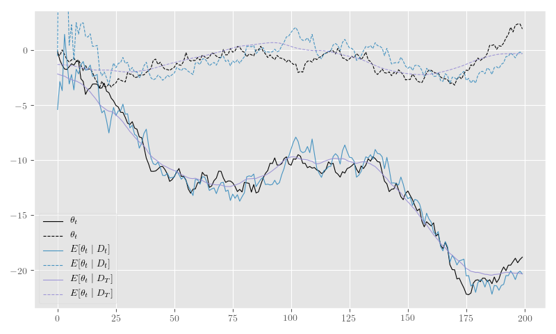
Forward-filtering Backward-sampling
We can use the smoothing and filtering steps in the previous section to perform more efficient MCMC estimation than would otherwise be possible without the Rao-Blackwellization inherent to both steps.
Forward-filtering backward-sampling (Fr-Schnatter 1994) works by first computing the forward filtered moments, allowing one to draw \(\theta_T\) from \(\left(\theta_T \mid D_T\right) \sim \operatorname{N}\left(m_T, C_T\right)\) and, subsequently, \(\theta_t\) from \(\left(\theta_t \mid \theta_{t+1}, D_T \right) \sim \operatorname{N}\left(h_t, H_t\right)\).
The latter distribution’s moments are easily derived from the filtered and smoothed moments:
\[\begin{equation} \begin{gathered} h_t = m_t + B_t \left(\theta_{t+1} - a_{t+1}\right) \\ H_t = C_t - B_t R_{t+1} B^\top_t \end{gathered} \label{eq:ffbs-moments} \end{equation}\]
Since all the quantities in \(\eqref{eq:ffbs-moments}\) appear in the filtering and smoothing moments, we can use the SVD-based approach described earlier to perform the updates and sampling. We reproduce the relevant subset of calculations in Listing 10.
def ffbs_step(m_t, U_C_t, S_C_t, a_tp1, U_R_tp1, S_R_tp1, theta_tp1, F_tp1, G_tp1, N_W_tp1_inv, rng):
    """Perform forward-filtering backward-sampling."""

    S_C_t_inv = tt_finite_inv(S_C_t)

    # H_t_inv = U_C_t @ N_H_t_inv.T @ N_H_t_inv @ U_C_t.T = G_tp1^T @ W_tp1_inv @ G_tp1.T + C_t_inv
    N_H_t_inv = tt.join(0,
                        matrix_dot(N_W_tp1_inv, G_tp1, U_C_t),
                        S_C_t_inv)
    _, d_N_H_t_inv, V_N_H_t_inv_T = svd(N_H_t_inv)

    U_H_t = U_C_t.dot(V_N_H_t_inv_T.T)
    s_H_t = tt_finite_inv(d_N_H_t_inv)

    N_C_t = S_C_t.dot(U_C_t.T)

    S_R_tp1_inv = tt_finite_inv(S_R_tp1)
    N_R_tp1_inv = S_R_tp1_inv.dot(U_R_tp1.T)

    # B_t = C_t @ G_tp1.T @ inv(R_tp1)
    # B_t = matrix_dot(U_H_t * s_H_t, s_H_t * U_H_t.T,
    #                  G_tp1.T, N_W_tp1_inv.T, N_W_tp1_inv)
    B_t = matrix_dot(N_C_t.T, N_C_t, G_tp1.T, N_R_tp1_inv.T, N_R_tp1_inv)

    h_t = m_t + B_t.dot(theta_tp1 - a_tp1)
    h_t.name = 'h_t'

    # TODO: Add an option or optimization to use the SVD to sample in
    # `MvNormalRV`.
    # theta_t = MvNormalRV(h_t, H_t, rng=rng, name='theta_t_ffbs')
    theta_t = h_t + tt.dot(U_H_t, s_H_t *
                           MvNormalRV(tt.zeros_like(h_t),
                                      tt.eye(h_t.shape[0]),
                                      rng=rng))

    # These are statistics we're gathering for other posterior updates
    theta_tp1_diff = theta_tp1 - G_tp1.dot(theta_t)
    f_tp1 = F_tp1.T.dot(theta_t)

    # Sequentially sample/update quantities conditional on `theta_t` here...

    return [theta_t, theta_tp1_diff, f_tp1]


# C_T = matrix_dot(U_C_T, tt.square(S_C_T), U_C_T.T)
# theta_T_post = MvNormalRV(m_T, C_T, rng=rng_tt)
theta_T_post = m_T + matrix_dot(U_C_T, S_C_T,
                                MvNormalRV(tt.zeros_like(m_T),
                                           tt.eye(m_T.shape[0]),
                                           rng=rng_tt))
theta_T_post.name = "theta_T_post"


ffbs_output, ffbs_updates = theano.scan(fn=ffbs_step,
                                        sequences=[
                                            {"input": m_t, "taps": [-1]},
                                            {"input": U_C_t, "taps": [-1]},
                                            {"input": S_C_t, "taps": [-1]},
                                            {"input": a_t, "taps": [1]},
                                            {"input": U_R_t, "taps": [1]},
                                            {"input": S_R_t, "taps": [1]}
                                        ],
                                        outputs_info=[
                                            {"initial": theta_T_post, "taps": [-1]},
                                            {}, {}, # theta_tp1_diff, f_tp1
                                        ],
                                        non_sequences=[F_tt, G_tt, N_W_inv_tt, rng_tt],
                                        go_backwards=True,
                                        strict=True,
                                        name='ffbs_samples')

(theta_t_post_rev, theta_t_diff_rev, f_t_rev) = ffbs_output

theta_t_post = tt.join(0, theta_t_post_rev[::-1], [theta_T_post])

# We need to add the missing end-points onto these statistics...
f_t_post = tt.join(0, f_t_rev[::-1], [F_tt.T.dot(theta_T_post)])Quantities besides the state values, \(\theta_t\), can be sampled sequentially (i.e. within the function ffbs_step in Listing 10), or after FFBS when all \(\theta_t \mid D_T\) have been sampled. These quantities can use the conditionally Gaussian form of \(\left(\theta_t \mid \theta_{t+1}, D_T \right)\) to derive Gibbs steps, further Rao-Blackwellize hierarchical quantities, or apply any other means of producing posterior samples conditional on \(\left(\theta_t \mid \theta_{t+1}, D_T \right)\).
In our simulation example, we will further augment our original model by adding the classic conjugate gamma priors to our previously fixed state and observation precision parameters, \(\phi_W\) and \(\phi_V\), respectively:
\[\begin{equation} \begin{gathered} \phi_{W} \sim \operatorname{Gamma}\left( a_W, b_W \right) ,\quad \phi_{V} \sim \operatorname{Gamma}\left( a_V, b_V \right) \end{gathered} \label{eq:phi-gamma-priors} \end{equation}\]
This classical conjugate prior allows one to derive simple closed-form posteriors for a Gibbs sampler conditional on \(y_t\), \(\theta_t\), and \(\theta_{t-1}\), as follows:
\[\begin{equation} \begin{gathered} \phi_{W} \mid D_T \sim \operatorname{Gamma}\left( a_W + \frac{N}{2}, b_W + \frac{1}{2} \sum_{t=1}^N \left( \theta_t - G_t \theta_{t-1} \right)^2 \right) ,\quad \phi_{V} \mid D_T \sim \operatorname{Gamma}\left( a_V + \frac{N}{2}, b_V + \frac{1}{2} \sum_{t=1}^N \left( y_t - F_t^\top \theta_t \right)^2 \right) \end{gathered} \label{eq:phi-gamma-posteriors} \end{equation}\]
Those posterior computations are implemented in Listings 11 and 12, and they are used to update the shared Theano variables for \(\phi_W\) and \(\phi_V\) within a Gibbs sampling loop in Listing 13.
Simulation Example
phi_W_a, phi_W_b = theano.shared(np.r_[2.5, 2.5]), theano.shared(np.r_[0.5, 0.5])

phi_W_a_post_tt = phi_W_a + N_obs_tt * 0.5
phi_W_SS_tt = tt.square(theta_t_diff_rev).sum(0)
phi_W_b_post_tt = phi_W_b + 0.5 * phi_W_SS_tt
phi_W_post_tt = GammaRV(phi_W_a_post_tt, phi_W_b_post_tt, rng=rng_tt, name='phi_W_post')phi_V_a, phi_V_b = theano.shared(0.125), theano.shared(0.25)
phi_V_a_post_tt = phi_V_a + N_obs_tt * 0.5
phi_V_SS_tt = tt.square(y_tt - f_t_post).sum()
phi_V_b_post_tt = phi_V_b + 0.5 * phi_V_SS_tt
phi_V_post_tt = GammaRV(phi_V_a_post_tt, phi_V_b_post_tt, rng=rng_tt, name='phi_V_post')ffbs_dlm = tt_function([y_tt, N_obs_tt, N_theta_tt, G_tt, F_tt],
[theta_t_post, phi_W_post_tt, phi_V_post_tt,
phi_W_SS_tt, phi_V_SS_tt],
updates=ffbs_updates)
rng_tt.get_value(borrow=True).set_state(rng_sim_state)
phi_W_0 = phi_W_a.get_value()/phi_W_b.get_value()
phi_V_0 = phi_V_a.get_value()/phi_V_b.get_value()
phi_W_tt.set_value(phi_W_0)
phi_V_tt.set_value(phi_V_0)
chain = 0
theta_label = r'$\theta_t \mid D_T$'
phi_W_label = r'$\phi_W \mid D_T$'
phi_V_label = r'$\phi_V \mid D_T$'
theta_t_post_sim, phi_W_post_sim, phi_V_post_sim = None, None, None
posterior_samples = {theta_label: [[]], phi_W_label: [[]], phi_V_label: [[]]}
for i in range(1000):
theta_t_post_sim, phi_W_post_sim, phi_V_post_sim, phi_W_SS_sim, phi_V_SS_sim = ffbs_dlm(
y_sim,
dlm_sim_values[N_obs_tt], dlm_sim_values[N_theta_tt],
dlm_sim_values[G_tt], dlm_sim_values[F_tt])
# Update variance precision parameters
phi_W_tt.set_value(phi_W_post_sim)
phi_V_tt.set_value(phi_V_post_sim)
posterior_samples[theta_label][chain].append(theta_t_post_sim)
posterior_samples[phi_W_label][chain].append(phi_W_post_sim)
posterior_samples[phi_V_label][chain].append(phi_V_post_sim)
print(f'i={i},\tphi_W={phi_W_post_sim}\t({phi_W_SS_sim}),\tphi_V={phi_V_post_sim} ({phi_V_SS_sim})')
posterior_samples = {k: np.asarray(v) for k,v in posterior_samples.items()}Figure 14 shows the posterior \(\theta_t\) samples and Figure 15 plots the posterior sample traces.
plt.clf()

fig, ax = plt.subplots(figsize=(8, 4.8))
ax.autoscale(enable=False)

# bivariate_cycler =  cycler('linestyle', ['-', '--']) * plt_orig_cycler
# ax.set_prop_cycle(bivariate_cycler)

thetas_shape = posterior_samples[theta_label][0].shape

cycle = ax._get_lines.prop_cycler

bivariate_obs_cycler =  cycler('linestyle', ['-', '--']) * cycler('color', ['black'])

ax.set_prop_cycle(bivariate_obs_cycler)
ax.plot(theta_t_sim, label=r'$\theta_t$', linewidth=1.0)

ax.autoscale(enable=True)
ax.autoscale(enable=False)

for d in range(thetas_shape[-1]):

    styles = next(cycle)
    thetas = posterior_samples[theta_label][0].T[d].T

    theta_lines = np.empty(thetas_shape[:-1] + (2,))
    theta_lines.T[0] = np.tile(np.arange(thetas_shape[-2]), [thetas_shape[-3], 1]).T
    theta_lines.T[1] = thetas.T

    ax.add_collection(
        LineCollection(theta_lines,
                       label=theta_label,
                       alpha=0.3, linewidth=0.9,
                       **styles)
    )

plt.tight_layout()

plt.legend(framealpha=0.4)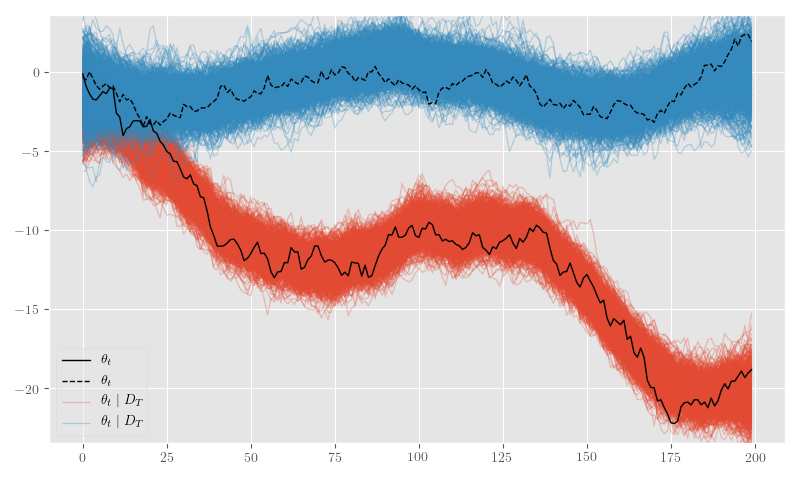
import arviz as az

az_trace = az.from_dict(posterior=posterior_samples)
az.plot_trace(az_trace, compact=True)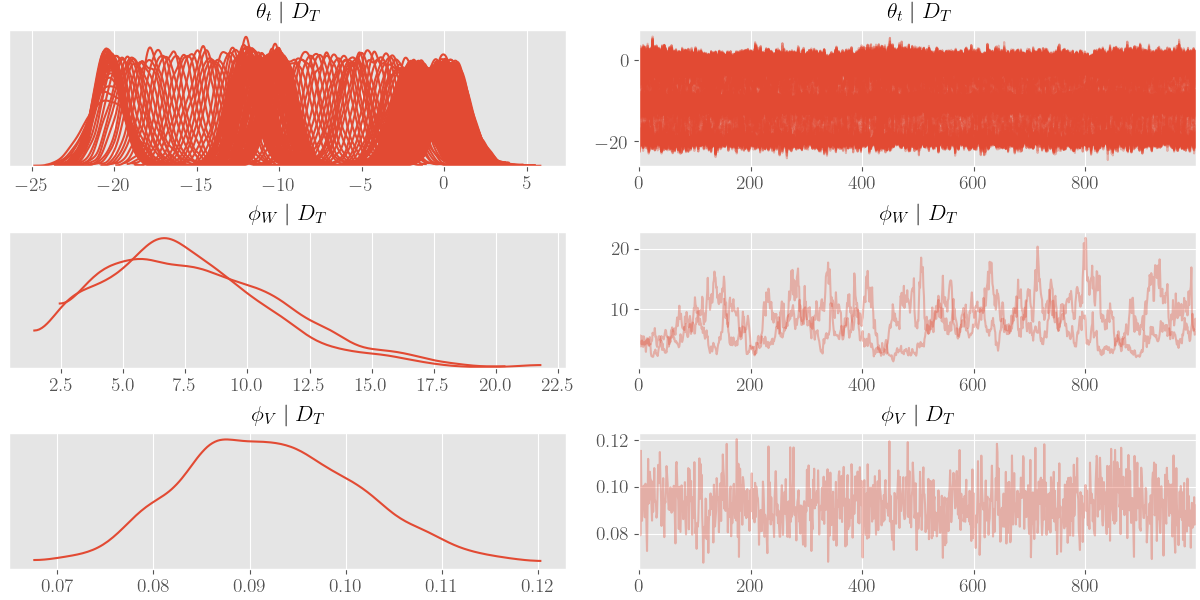
plt.close('all')

fig, ax = plt.subplots(figsize=(8, 4.8))

ax.plot(y_sim, label=r'$y_t$', linewidth=1.0, color='black')

ax.autoscale(enable=True)
ax.autoscale(enable=False)

f_t_ordinates = np.dot(posterior_samples[theta_label][0], dlm_sim_values[F_tt].squeeze())

f_t_lines = np.empty(f_t_ordinates.shape + (2,))
f_t_lines.T[0] = np.tile(np.arange(f_t_ordinates.shape[1]), [f_t_ordinates.shape[0], 1]).T
f_t_lines.T[1] = f_t_ordinates.T

ax.add_collection(
    LineCollection(f_t_lines,
                   label=r'$E[y_t \mid \theta_t, D_T]$',
                   alpha=0.3, linewidth=0.9, color='red')
)

plt.tight_layout()

plt.legend(framealpha=0.4)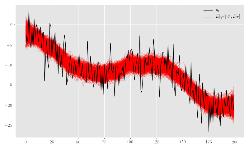
Non-Gaussian Extension
Let’s say we want to model count observations that are driven by a smooth time-varying process. We can assume a negative-binomial observation model with a log-link function–in standard GLM fashion (McCullagh & Nelder 1989)–and connect it to the same state and observation dynamics as the basic DLM in \(\eqref{eq:basic-dlm-state}\) via its mean \(\mu_t = \exp\left(\eta_t\right)\):
\[\begin{equation} \begin{aligned} Y_t &\sim \operatorname{NB}\left(r, p_t\right) \\ E[Y_t \mid \theta_t] &= \mu_t = \exp\left( F_t^\top \theta_t \right) \\ \theta_t &= G_t \theta_{t-1} + \nu_t, \quad \nu_t \sim \operatorname{N}\left( 0, W \right) \end{aligned} \label{eq:nb-dlm} \end{equation}\]
Under the parameterization \(p_t = \frac{\mu_t}{\mu_t + r}\), the negative-binomial density function takes the following form:
\[\begin{equation} \begin{aligned} \operatorname{p}\left(Y_t = y_t \mid r, p_t\right) &= \frac{\Gamma\left( y_t + r \right)}{y_t!\,\Gamma(r)} \left( 1 - p_t \right)^r \left( p_t \right)^{y_t} \\ &= \frac{\Gamma\left( y_t + r \right)}{y_t!\,\Gamma(r)} \left( \frac{r}{r + \mu_t} \right)^r \left( \frac{\mu_t}{r + \mu_t} \right)^{y_t} \\ &= \frac{\Gamma\left( y_t + r \right)}{y_t!\,\Gamma(r)} \frac{\left( \mu_t / r \right)^{y_t}}{\left( 1 + \mu_t / r \right)^{r + y_t}} \\ &= \frac{\Gamma\left( y_t + r \right)}{y_t!\,\Gamma(r)} \frac{\left( e^{\eta_t - \log r} \right)^{y_t}}{\left( 1 + e^{\eta_t - \log r} \right)^{r + y_t}} . \end{aligned} \label{eq:nb-pmf} \end{equation}\]
The logit-inverse form in \(\eqref{eq:nb-pmf}\) has a Gaussian scale-mixture representation in the Pólya-Gamma distribution (Polson, Scott & Windle 2013). Said scale-mixture is as follows:
\[\begin{equation} \begin{aligned} \frac{e^{\psi a}}{\left(1 + e^{\psi}\right)^b} &= 2^{-b} e^{\kappa \psi} \int^{\infty}_{0} e^{-\frac{\omega}{2} \psi^2} \operatorname{p}(\omega) d\omega \\ &= 2^{-b} \int^{\infty}_{0} e^{-\frac{\omega}{2} \left( \psi - \frac{\kappa}{\omega} \right)^2} e^{\frac{\kappa^2}{2 \omega} } \operatorname{p}(\omega) d\omega . \end{aligned} \label{eq:pg-identity} \end{equation}\]
where \(\kappa = a - b / 2\) and \(\omega_t \sim \operatorname{PG}\left(b, 0\right)\).
When the Gaussian scale-mixture identity of \(\eqref{eq:pg-identity}\) is applied to our observation model in \(\eqref{eq:nb-pmf}\), \(a = y_t\), \(b = r + y_t\), \(\kappa = (y_t - r)/2\), and \(\psi = \eta_t - \log r\).
From the scale mixture formulation, we obtain the following augmented joint observation model density:
\[\begin{equation} \begin{aligned} \operatorname{p}(\theta_t \mid \omega, y_t, r, D_{t-1}) &\propto \exp\left(-\frac{\omega}{2} \left( F_t^\top \theta_t - \left( \log r + \frac{y_t - r}{2 \omega} \right) \right)^2 \right) \operatorname{p}(\theta_t \mid D_{t-1}) \\ &= e^{-\frac{\omega}{2} \left(y^*_t - F_t^\top \theta_t \right)^2} \operatorname{p}(\theta_t \mid D_{t-1}) \\ &\propto \operatorname{p}\left( y^*_t \mid F_t^\top \theta_t, \omega^{-1} \right) \operatorname{p}(\theta_t \mid D_{t-1}) \end{aligned} \label{eq:nb-aug-obs} \end{equation}\]
where \(y^*_t = \log r + \frac{y_t - r}{2 \omega}\).
The reformulation at the end of \(\eqref{eq:nb-aug-obs}\) characterizes a distribution of “virtual” observations,
\[\begin{equation} y^*_t = F_t^\top \theta_t + \epsilon^*_t,\quad \epsilon^*_t \sim \operatorname{N}\left(0, V^*_t \right) , \label{eq:nb-virtual-obs} \end{equation}\]
with \(V_t = \operatorname{diag}\left( \omega^{-1}_t \right)\).
The augmented observation equation in \(\eqref{eq:nb-virtual-obs}\) recovers our original DLM formulation in \(\eqref{eq:basic-dlm-obs}\) and–by comparison–details the changes needed to use the Pólya-Gamma scale-mixture. Specifically, we need to sample \(\omega_t \sim \operatorname{PG}\left(r + y_t, F_t^\top \theta_t - \log r \right)\) and perform the following substitutions: \(y_t \to y^*_t\) and \(V_t \to V^*_t\).
Simulation Example
Listing 17 creates a Theano graph for negative-binomial model defined in \(\eqref{eq:nb-dlm}\).
from symbolic_pymc.theano.random_variables import NegBinomialRV


r_tt = tt.iscalar('r')


def nb_obs_step(theta_t, F_t, r, rng):
    mu_t = tt.exp(F_t.T.dot(theta_t))
    p_t = mu_t / (mu_t + r)
    y_t = NegBinomialRV(r, (1. - p_t), rng=rng, name='y_t')
    return y_t, p_t


nb_obs_res, nb_Y_t_updates = theano.scan(fn=nb_obs_step,
                                         sequences=[theta_t_rv],
                                         non_sequences=[F_tt, r_tt, rng_tt],
                                         outputs_info=[
                                             {}, {}, # y_t, p_t
                                         ],
                                         strict=True,
                                         name='Y_t')

nb_Y_t_rv, nb_p_t_tt = nb_obs_res
Listing 18 specifies parameters for a simulation from \(\eqref{eq:nb-dlm}\) and samples a series.
nb_dlm_sim_values = dlm_sim_values.copy()
nb_dlm_sim_values[F_tt] = np.array([[1.0],
                                    [0.0]], dtype=theano.config.floatX)
nb_dlm_sim_values[G_tt] = np.array([[1.0, 0.1],
                                    [0.0, 0.8]], dtype=theano.config.floatX)
nb_dlm_sim_values[r_tt] = 1000

phi_W_tt.set_value(np.r_[10.0, 10.0])

rng_tt.get_value(borrow=True).set_state(rng_init_state)

simulate_nb_dlm = tt_function([N_obs_tt, N_theta_tt, G_tt, F_tt, r_tt],
                              [nb_Y_t_rv, theta_t_rv, nb_p_t_tt],
                              givens={theta_0_rv: np.r_[1.0, 0.5]},
                              updates=nb_Y_t_updates)

sim_nb_res = simulate_nb_dlm(nb_dlm_sim_values[N_obs_tt],
                             nb_dlm_sim_values[N_theta_tt],
                             nb_dlm_sim_values[G_tt],
                             nb_dlm_sim_values[F_tt],
                             nb_dlm_sim_values[r_tt])

nb_y_sim, nb_theta_t_sim, nb_p_t_sim = sim_nb_resIn Figure 19 we plot the sample generated in Listing 17.
plt.clf()

fig, ax = plt.subplots(figsize=(8, 4.8))
_ = ax.plot(nb_y_sim, label=r'$y_t$', color='black', linewidth=1.2, drawstyle='steps-pre')

plt.tight_layout()
plt.legend()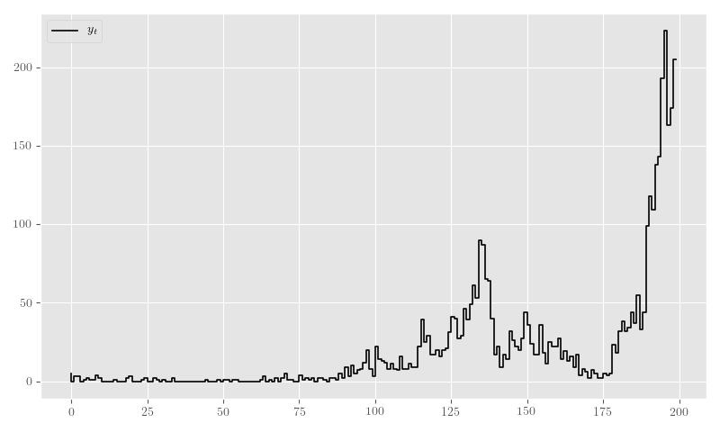
plt.clf()

fig, ax = plt.subplots(figsize=(8, 4.8))
ax.autoscale(enable=False)

bivariate_obs_cycler =  cycler('linestyle', ['-', '--']) * cycler('color', ['black'])

ax.set_prop_cycle(bivariate_obs_cycler)
ax.plot(nb_theta_t_sim, label=r'$\theta_t$', linewidth=1.0)

ax.autoscale(enable=True)

plt.tight_layout()

plt.legend(framealpha=0.4)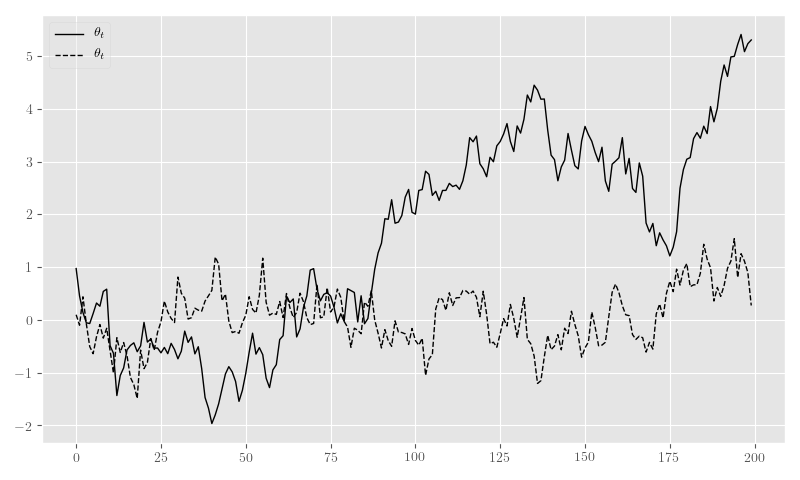
plt.clf()

fig, ax = plt.subplots(figsize=(8, 4.8))

ax.plot(nb_p_t_sim, label=r'$p_t$', linewidth=1.0, color='black')

plt.tight_layout()
plt.legend(framealpha=0.4)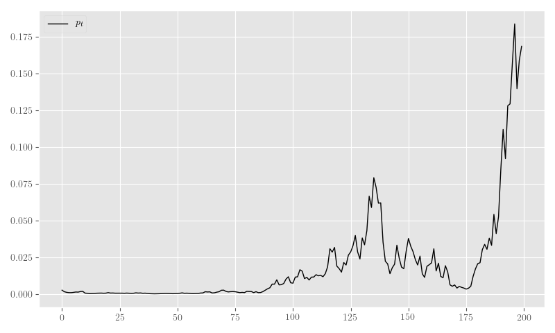
Augmented FFBS Sampler
In order to create a FFBS sampler for our Pólya-Gamma DLM in \(\eqref{eq:nb-aug-obs}\), we need to update the filtering code to use time-varying “virtual” observation variances, \(V^*_t\). After this change is made, all Theano graphs that depend on the resulting objects need to be recreated, as well. This is done in Listing 22.
V_t_tt = tt.specify_shape(tt.col(), [N_obs_tt, 1])
V_t_tt.name = 'V_t'


def nb_filtering_step(y_t, V_t, m_tm1, U_C_tm1, S_C_tm1, F_t, G_t, N_W_t):
    N_V_t_inv = tt.diag(tt_finite_inv(tt.sqrt(V_t), eps_truncate=True))
    return filtering_step(y_t, m_tm1, U_C_tm1, S_C_tm1, F_t, G_t, N_W_t, N_V_t_inv)


filter_res, filter_updates = theano.scan(fn=nb_filtering_step,
                                         sequences=[y_tt, V_t_tt],
                                         outputs_info=[
                                             {"initial": m_0_tt, "taps": [-1]},
                                             {"initial": U_C_0_tt, "taps": [-1]},
                                             {"initial": S_C_0_tt, "taps": [-1]},
                                             {}, {}, {}  # a_t, U_R_t, S_R_t
                                         ],
                                         non_sequences=[F_tt, G_tt, N_W_tt],
                                         strict=True,
                                         name='theta_filtered')

(m_t, U_C_t, S_C_t, a_t, U_R_t, S_R_t) = filter_res

m_T = m_t[-1]
U_C_T = U_C_t[-1]
S_C_T = S_C_t[-1]

C_T = matrix_dot(U_C_T, tt.square(S_C_T), U_C_T.T)
theta_T_post = MvNormalRV(m_T, C_T, rng=rng_tt)
theta_T_post.name = "theta_T_post"

ffbs_output, ffbs_updates = theano.scan(fn=ffbs_step,
                                        sequences=[
                                            {"input": m_t, "taps": [-1]},
                                            {"input": U_C_t, "taps": [-1]},
                                            {"input": S_C_t, "taps": [-1]},
                                            {"input": a_t, "taps": [1]},
                                            {"input": U_R_t, "taps": [1]},
                                            {"input": S_R_t, "taps": [1]}
                                        ],
                                        outputs_info=[
                                            {"initial": theta_T_post, "taps": [-1]},
                                            {}, {}, # theta_tp1_diff, f_tp1
                                        ],
                                        non_sequences=[F_tt, G_tt, N_W_inv_tt, rng_tt],
                                        go_backwards=True,
                                        strict=True,
                                        name='ffbs_samples')

(theta_t_post_rev, theta_t_diff_rev, f_t_rev) = ffbs_output

theta_t_post = tt.join(0, theta_t_post_rev[::-1], [theta_T_post])

f_t_post = tt.join(0, f_t_rev[::-1], [F_tt.T.dot(theta_T_post)])phi_W_a_post_tt = phi_W_a + N_obs_tt * 0.5
phi_W_b_post_tt = phi_W_b + 0.5 * tt.square(theta_t_diff_rev).sum(0)
phi_W_post_tt = GammaRV(phi_W_a_post_tt, phi_W_b_post_tt, rng=rng_tt, name='phi_W_post')Simulation Example
In Listing 24 we sample the initial values and create Theano terms for posterior/updated \(\omega_t\)-related values.
from pypolyagamma import PyPolyaGamma

from symbolic_pymc.theano.random_variables import PolyaGammaRV


y_raw_tt = theano.shared(nb_y_sim.astype(theano.config.floatX), name='y_raw_t')

r_sim = np.array(nb_dlm_sim_values[r_tt], dtype='double')

# XXX: testing
F_t_theta_0 = np.dot(nb_theta_t_sim, nb_dlm_sim_values[F_tt])

omega_0 = np.empty(nb_y_sim.shape[0], dtype='double')
PyPolyaGamma(12344).pgdrawv(r_sim + nb_y_sim.squeeze(),
                            F_t_theta_0.squeeze() - np.log(r_sim),
                            omega_0)
omega_0 = np.expand_dims(omega_0, -1)

y_aug_0 = np.log(r_sim) + (nb_y_sim - r_sim) / (2.0 * omega_0)

omega_t_tt = theano.shared(omega_0, name='omega_t')

omega_post_tt = PolyaGammaRV(r_tt + y_raw_tt, theta_t_post.dot(F_tt) - tt.log(r_tt), rng=rng_tt, name='omega_post')

y_aug_post_tt = tt.log(r_tt) + (y_raw_tt - r_tt) / (2.0 * omega_post_tt)
y_aug_post_tt.name = 'y_aug_post'Finally, the sampler steps are defined and executed in Listing 25.
nb_ffbs_dlm = tt_function([N_obs_tt, N_theta_tt, y_tt, G_tt, F_tt, V_t_tt, r_tt],
                          [theta_t_post, phi_W_post_tt, omega_post_tt, y_aug_post_tt],
                          updates=ffbs_updates)

rng_tt.get_value(borrow=True).set_state(rng_sim_state)

phi_W_tt.set_value(np.r_[10.0, 10.0])

chain = 0

theta_label = r'$\theta_t \mid D_T$'
phi_W_label = r'$\phi_W \mid D_T$'
omega_label = r'$\omega_t \mid D_T$'

theta_t_post_sim, phi_W_post_sim, omega_post_sim, y_aug_post_sim = None, None, None, None
nb_posterior_samples = {theta_label: [[]], phi_W_label: [[]], omega_label: [[]]}

V_t_sim = np.reciprocal(omega_0)
y_aug_sim = y_aug_0

for i in range(1000):

    nb_ffbs_res = nb_ffbs_dlm(
        nb_dlm_sim_values[N_obs_tt],
        nb_dlm_sim_values[N_theta_tt],
        y_aug_sim,
        nb_dlm_sim_values[G_tt],
        nb_dlm_sim_values[F_tt],
        V_t_sim,
        nb_dlm_sim_values[r_tt])

    theta_t_post_sim, phi_W_post_sim, omega_post_sim, y_aug_post_sim = nb_ffbs_res

    phi_W_tt.set_value(phi_W_post_sim)
    omega_t_tt.set_value(omega_post_sim)

    V_t_sim = np.reciprocal(omega_post_sim)
    y_aug_sim = y_aug_post_sim

    nb_posterior_samples[theta_label][chain].append(theta_t_post_sim)
    nb_posterior_samples[phi_W_label][chain].append(phi_W_post_sim)
    nb_posterior_samples[omega_label][chain].append(omega_post_sim)

    print(f'i={i},\tphi_W={phi_W_post_sim}')

nb_posterior_samples = {k: np.asarray(v) for k,v in nb_posterior_samples.items()}Figure 26 shows the posterior \(\theta_t\) samples, Figure 27 plots the posterior sample traces, and Figure 28 shows \(p_t \mid \theta_t\).
plt.clf()

fig, ax = plt.subplots(figsize=(8, 4.8))
ax.autoscale(enable=False)

thetas_shape = nb_posterior_samples[theta_label][0].shape

cycle = ax._get_lines.prop_cycler

bivariate_obs_cycler =  cycler('linestyle', ['-', '--']) * cycler('color', ['black'])

ax.set_prop_cycle(bivariate_obs_cycler)
ax.plot(nb_theta_t_sim, label=r'$\theta_t$', linewidth=1.0)

ax.autoscale(enable=True)
ax.autoscale(enable=False)

for d in range(thetas_shape[-1]):

    styles = next(cycle)
    thetas = nb_posterior_samples[theta_label][0].T[d].T

    theta_lines = np.empty(thetas_shape[:-1] + (2,))
    theta_lines.T[0] = np.tile(np.arange(thetas_shape[-2]), [thetas_shape[-3], 1]).T
    theta_lines.T[1] = thetas.T

    ax.add_collection(
        LineCollection(theta_lines,
                       label=theta_label,
                       alpha=0.05, linewidth=0.9,
                       **styles)
    )

plt.tight_layout()

plt.legend(framealpha=0.4)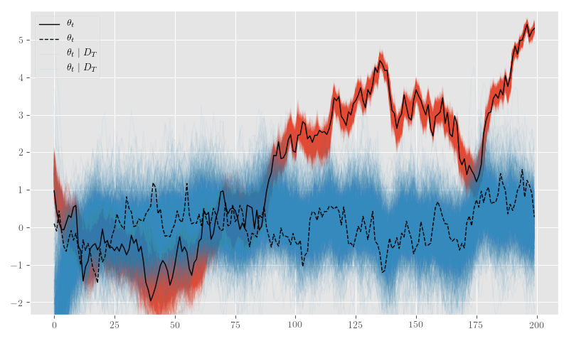
import arviz as az

az_trace = az.from_dict(posterior=nb_posterior_samples)
az.plot_trace(az_trace, compact=True)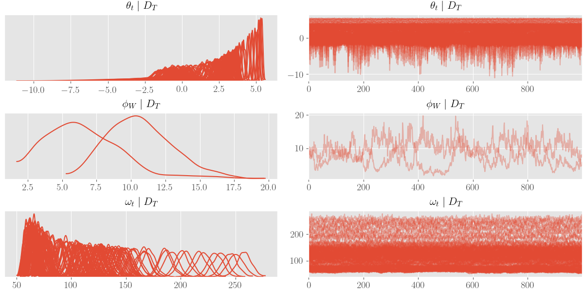
plt.close('all')

fig, ax = plt.subplots(figsize=(8, 4.8))

ax.plot(nb_p_t_sim, label=r'$p_t$', linewidth=1.0, color='black')

ax.autoscale(enable=True)
ax.autoscale(enable=False)

mu_t_sim = np.exp(np.dot(nb_posterior_samples[theta_label][0], nb_dlm_sim_values[F_tt].squeeze()))
p_t_sim = mu_t_sim / (mu_t_sim + nb_dlm_sim_values[r_tt])

p_t_lines = np.empty(p_t_sim.shape + (2,))
p_t_lines.T[0] = np.tile(np.arange(p_t_sim.shape[1]), [p_t_sim.shape[0], 1]).T
p_t_lines.T[1] = p_t_sim.T

ax.add_collection(
    LineCollection(p_t_lines,
                   label=r'$p_t \mid \theta_t, D_T$',
                   alpha=0.3, linewidth=0.9, color='red')
)

plt.tight_layout()

plt.legend(framealpha=0.4)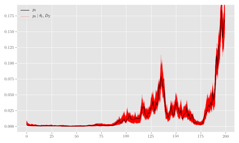
COVID–19 Example
As another example, we’ll use data from the COVID–19 outbreak in New York and we’ll only concentrate on the positive test counts. We do not make any assertions about the results; we simply want to apply our implementation to a real-life dataset. If anything, we would simply like to highlight the potential provided by these flexible and constructive Bayesian frameworks and offer a concrete starting point for motivated statisticians and Python developers.
To start, Listing 29 pulls and formats the COVID–19 data and Figure 30 plots it.
import pandas as pd


url = 'https://covidtracking.com/api/v1/states/daily.csv'
states = pd.read_csv(url, parse_dates=['date'], index_col=['state','date']).sort_index()
state = 'NY'

counts = states.loc[state, ['positive', 'total']].diff().loc['2020-03-20':]
counts.columns = ['new_positive_tests', 'new_total_tests']plt.clf()
fig, ax = plt.subplots(figsize=(8, 4.8))
_ = ax.plot(counts.new_positive_tests, label=r'$y_t$', color='black', linewidth=1.2, drawstyle='steps-pre')
plt.tight_layout()
plt.legend()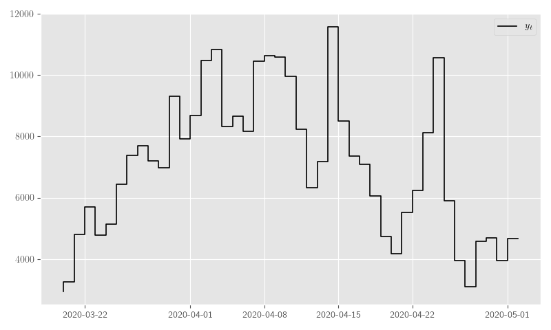
Our example model is a simple Gaussian walk with an unknown evolution variance (i.e. again, modeled by a gamma prior on the precision \(\phi_W\)) given by the following values:
\[\begin{equation} \begin{gathered} F_t = \begin{pmatrix} 1 \end{pmatrix} ,\quad G_t = \begin{pmatrix} 1 \end{pmatrix} \\ W_t = \begin{pmatrix} \phi_{W}^{-1} \end{pmatrix} , \quad \phi_{W} \sim \operatorname{Gamma}\left(2.5, 0.5\right) , \quad \phi_{W} = 10 \end{gathered} \label{eq:ny-model-settings} \;. \end{equation}\]
Again, we set \(r = 1000\), effectively making our negative-binomial a Poisson approximation. Listing 31 sets the initial values in \(\eqref{eq:ny-model-settings}\) and Listing 32 specifies the sampler loop.
nb_dlm_ny_values = {
    N_obs_tt: counts.new_positive_tests.shape[0],
    N_theta_tt: 1
}
nb_dlm_ny_values[F_tt] = np.array([[1.0]], dtype=theano.config.floatX)
nb_dlm_ny_values[G_tt] = np.array([[1.0]], dtype=theano.config.floatX)
nb_dlm_ny_values[r_tt] = 1000

phi_W_a.set_value(np.r_[2.5])
phi_W_b.set_value(np.r_[0.5])
phi_W_tt.set_value(np.r_[10.0])

rng_tt.get_value(borrow=True).set_state(rng_init_state)

y_raw_tt.set_value(np.expand_dims(counts.new_positive_tests, -1).astype(theano.config.floatX))

r_ny = np.array(nb_dlm_ny_values[r_tt], dtype='double')

omega_0 = np.empty(counts.new_positive_tests.shape[0], dtype='double')
PyPolyaGamma(12344).pgdrawv(r_ny + counts.new_positive_tests.values,
                            F_t_theta_0.squeeze() - np.log(r_ny),
                            omega_0)
omega_0 = np.expand_dims(omega_0, -1)

y_aug_0 = np.log(r_ny) + (counts.new_positive_tests.values[:, np.newaxis] - r_ny) / (2.0 * omega_0)

omega_t_tt.set_value(omega_0)nb_ffbs_dlm = tt_function([N_obs_tt, N_theta_tt, y_tt, G_tt, F_tt, V_t_tt, r_tt],
[theta_t_post, phi_W_post_tt, omega_post_tt, y_aug_post_tt],
# mode='FAST_COMPILE',
updates=ffbs_updates)
rng_tt.get_value(borrow=True).set_state(rng_sim_state)
chain = 0
theta_label = r'$\theta_t \mid D_T$'
phi_W_label = r'$\phi_W \mid D_T$'
omega_label = r'$\omega_t \mid D_T$'
theta_t_post_sim, phi_W_post_sim, omega_post_sim, y_aug_post_sim = None, None, None, None
nb_ny_posterior_samples = {theta_label: [[]], phi_W_label: [[]], omega_label: [[]]}
V_t_sim = np.reciprocal(omega_0)
y_aug_sim = y_aug_0
for i in range(5000):
nb_ffbs_res = nb_ffbs_dlm(
nb_dlm_ny_values[N_obs_tt],
nb_dlm_ny_values[N_theta_tt],
y_aug_sim,
nb_dlm_ny_values[G_tt],
nb_dlm_ny_values[F_tt],
V_t_sim,
nb_dlm_ny_values[r_tt])
theta_t_post_sim, phi_W_post_sim, omega_post_sim, y_aug_post_sim = nb_ffbs_res
phi_W_tt.set_value(phi_W_post_sim)
omega_t_tt.set_value(omega_post_sim)
V_t_sim = np.reciprocal(omega_post_sim)
y_aug_sim = y_aug_post_sim
nb_ny_posterior_samples[theta_label][chain].append(theta_t_post_sim)
nb_ny_posterior_samples[phi_W_label][chain].append(phi_W_post_sim)
nb_ny_posterior_samples[omega_label][chain].append(omega_post_sim)
print(f'i={i},\tphi_W={phi_W_post_sim}')
# Convert and thin samples
nb_ny_posterior_samples = {k: np.asarray(v)[:, 1000:] for k,v in nb_ny_posterior_samples.items()}import arviz as az
az_trace = az.from_dict(posterior=nb_ny_posterior_samples)
az.plot_trace(az_trace, compact=True)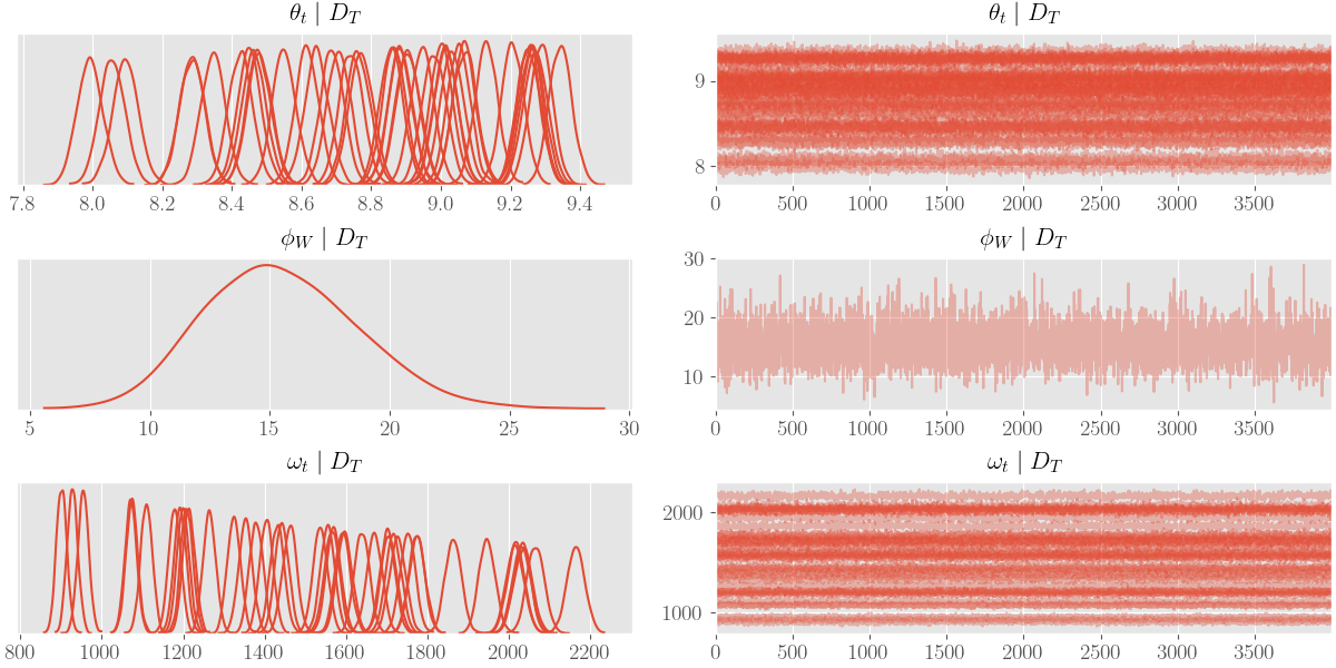
fig, ax = plt.subplots(figsize=(8, 4.8))

thetas_shape = nb_ny_posterior_samples[theta_label][0].shape

cycle = ax._get_lines.prop_cycler

bivariate_obs_cycler =  cycler('linestyle', ['-', '--']) * cycler('color', ['black'])

ax.set_prop_cycle(bivariate_obs_cycler)

for d in range(thetas_shape[-1]):

    styles = next(cycle)
    thetas = nb_ny_posterior_samples[theta_label][0].T[d].T

    theta_lines = np.empty(thetas_shape[:-1] + (2,))
    theta_lines.T[0] = np.tile(np.arange(thetas_shape[-2]), [thetas_shape[-3], 1]).T
    theta_lines.T[1] = thetas.T

    ax.add_collection(
        LineCollection(theta_lines,
                       label=theta_label,
                       alpha=0.05, linewidth=0.9,
                       **styles)
    )

ax.autoscale(enable=True)
plt.tight_layout()

plt.legend(framealpha=0.4)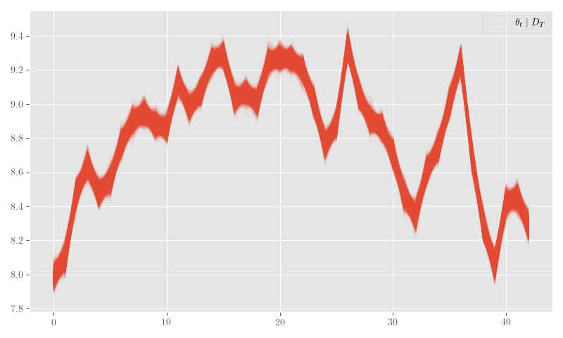
import scipy


plt.close('all')

fig, ax = plt.subplots(figsize=(8, 4.8))

ax.plot(counts.new_positive_tests.values, label=r'$y_t$', linewidth=1.0, color='black')

mu_t_sim = np.exp(np.dot(nb_ny_posterior_samples[theta_label][0], nb_dlm_ny_values[F_tt].squeeze()))
p_t_sim = mu_t_sim / (mu_t_sim + nb_dlm_ny_values[r_tt])

y_t_sim = scipy.stats.nbinom.rvs(nb_dlm_ny_values[r_tt], (1. - p_t_sim)).squeeze()

y_t_lines = np.empty(y_t_sim.shape + (2,))
y_t_lines.T[0] = np.tile(np.arange(y_t_sim.shape[1]), [y_t_sim.shape[0], 1]).T
y_t_lines.T[1] = y_t_sim.T

ax.add_collection(
    LineCollection(y_t_lines,
                   label=r'$y_t \mid \theta_t, D_T$',
                   alpha=0.3, linewidth=0.9, color='red'),
)

ax.autoscale(enable=True)
plt.tight_layout()

plt.legend(framealpha=0.4)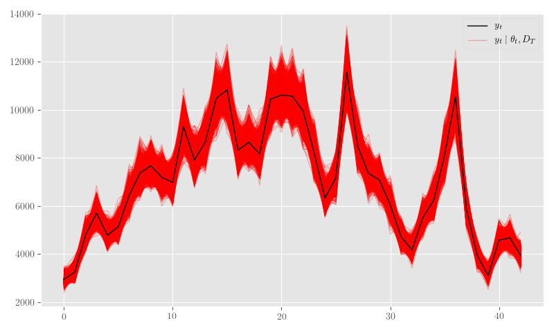
Discussion
We’ve implemented a highly extensible Bayesian timeseries framework with respectable model coverage (e.g. ARIMA models, polynomial trends, Fourier seasonality, dynamic regression, etc.), and shown how such a basic class can be extended to non-Gaussian observations. Additionally, we were able to show how an existing model-specialized sampler, i.e. FFBS, can be adapted alongside such an extension using the conditional linearity provided by a Gaussian scale-mixture.
In general, the same scale-mixture and conditional linearity techniques can be employed for other observation distributions (e.g. Beta, Binomial), as well as state-of-the-art shrinkage and sparsity priors (Bhadra, Datta, Polson & Willard 2016),(Datta & Dunson 2016).
Although we used Gibbs sampling, these techniques do not necessitate it; one can use Metropolis–or any other mathematically sound–steps instead.
Bayesian frameworks like these have considerable flexibility and are amenable to much analytic creativity; unfortunately, we don’t often see this–directly, at least–in practice. There are clearly some roadblocks to the average applied statistics/data science developer when attempting to implement these models straight from published papers. Those roadblocks often involve subtle numeric stability issues and a sometimes non-standard mathematics proficiency.
We hope that future automations will be able to address more straight-forward numerical stability issues by–for instance–automating the SVD-based reformulations used herein. The scale mixture manipulations are likewise amenable to certain automations, but, at the very least, it would serve the Bayesian community–and all who desire to construct non-trivial principled statistical models–well to develop low-level tools that codify and generate such scale-mixture variations. In this way, even experimentation by knowledgeable developers will be much easier and less error-prone.
Bibliography
Harrison & West, Bayesian Forecasting & Dynamic Models, Springer (1999). ↩︎
Petris, Petrone & Campagnoli, Dynamic Linear Models, Springer (2009). ↩︎
Gamerman & Lopes, Markov Chain Monte Carlo: Stochastic Simulation for Bayesian Inference, CRC Press (2006). ↩︎
Pole, West & Harrison, Applied Bayesian Forecasting and Time Series Analysis, CRC Press (1994). ↩︎
Bergstra, Breuleux, Bastien, Lamblin, Pascanu, Desjardins, Turian, Warde-Farley & Bengio, Theano: A CPU and GPU Math Expression Compiler, in in: Proceedings of the Python for Scientific Computing Conference (SciPy), edited by (2010) ↩︎
Willard, Symbolic-Pymc, , (2019). link. ↩︎
Zhang & Li, Fixed-Interval Smoothing Algorithm Based on Singular Value Decomposition, 916–921, in in: , Proceedings of the 1996 IEEE International Conference on Control Applications, 1996, edited by (1996) ↩︎
Petris, Petrone & Campagnoli, Dynamic Linear Models, Springer (2009). ↩︎
Fr"uhwirth-Schnatter, Data Augmentation and Dynamic Linear Models, Journal of time series analysis, 15(2), 183–202 (1994). link. ↩︎
McCullagh & Nelder, Generalized Linear Models, CRC press (1989). ↩︎
Polson, Scott & Windle, Bayesian Inference for Logistic Models Using P'olyaLatent Variables, Journal of the American Statistical Association, 108(504), 1339–1349 (2013). link. ↩︎
Bhadra, Datta, Polson & Willard, Default Bayesian analysis with global-local shrinkage priors, Biometrika, 103(4), 955–969 (2016). doi. ↩︎
Datta & Dunson, Bayesian Inference on Quasi-Sparse Count Data, Biometrika, 103(4), 971–983 (2016). ↩︎
Comments
comments powered by Disqus