Introduction
In this post I want to address some concepts regarding statistical model specification within the Bayesian paradigm, motivation for its use, and the utility of sample results (e.g. empirical posterior distributions). This write-up isn’t intended to be thorough or self-contained, especially since numerous quality introductions already exist for Bayesian modeling and MCMC (Gelman, Carlin, Stern, Dunson, Vehtari & Rubin 2013). Instead, its purpose is to illustrate some specific points in the context of a simple, evolving problem that mirrors some real-life objectives. Also, what’s advocated here is in large part just statistical modeling and not exclusively Bayesian.
The generality, applicability and relative simplicity of the core concepts within Bayesian modeling are sadly overlooked in practice. Bayes is too often conflated with MCMC and its associated computational costs, or is seen as needlessly “mathy” and technical. I argue that there is an oft unacknowledged trade-off in the efforts of mathematical modeling, and that Bayesian modeling helps navigate that complexity. In doing so, one can save on expended efforts in the long run.
When a model is [fully] specified in a statistical or Bayesian way, the modeler has at their disposal distributions for the unknown quantities of interest; these distributions are often the primary interest. The desired estimates are found “within” the distributions. For instance, as a distribution’s moments (e.g. mean, mode, variance, etc.), which may correspond to certain “best” estimates or measures of parameter uncertainty. The same goes for functions of these distributions (e.g. rolling sums and averages).
Normally, modeling objectives are specified in terms of point-estimates instead of distributions: like the aforementioned “best” parameter estimates. This situation is also covered by the Bayesian paradigm, especially when the corresponding distributions have a closed-form and are fully specified by a finite number of parameters. However, when this isn’t the case, point-estimates provide only part of the picture. It’s usually these missing parts that make model assessment and prediction largely separate and difficult endeavours down the road.
Even so, modeling and estimation often proceeds without much statistical consideration or context, making these distributions–and the results they can provide–more and more inaccessible. In a situation where modeling started with common machine learning/statistical software and resulted in non-statistical extensions, the work needed for something like uncertainty quantification or propagation broadly equates to retrofitting and/or defining the altered or missing statistical context of the problem. This sort of work necessarily requires a much rarer expertise, which is usually too difficult for outsiders to vet. Considerations like this might be reason enough to–at least minimally–maintain clear statistical assumptions throughout the life of a non-trivial project. The Bayesian approach can be a more accessible means of providing this type of statistical coherency.
As a starting point, one can find quite a few non-Bayes models with Bayesian interpretations and counterparts. Even finding a Bayesian interpretation for an existing non-Bayes model can itself advance one’s understanding of the statistical assumptions and properties of the model. In some cases this understanding can inspire new forms of estimation or new non-Bayes variants of a model. Multiple examples arise from models defined by objective or loss functions with forms equivalent to the total log-likelihoods of Bayesian models. This, for instance, is one way that general point-wise estimates can be related to maximum a posteriori (MAP) estimates in the Bayesian context.
Notation
Before getting into the details, let’s cover some preliminaries regarding notation.
The symbol \(\sim\) is overloaded to mean a couple things. First, a statement like \(X \sim \operatorname{P}\) means “\(X\) is distributed according to \(\operatorname{P}\)”, when \(X\) is understood to be a random variable (generally denoted by capital letter variables). Second, for a non-random variable \(x\), \(x \sim \operatorname{P}\) and \(x \sim X\) means “\(x\) is a sample from distribution \(\operatorname{P}\)”. When \(\operatorname{P}\) is not meant to signify a distribution, but instead a generic function–like a probability density function \(p(X=x) \equiv p(x)\), then the distribution in question is [the] one arising from the function (interpreted as a probability density and/or measure)–when possible. See here for a similar notation. Also, whenever indices are dropped, the resulting symbol is assumed to be a stacked matrix containing each entry, e.g.
\[\begin{gather*} X^\top = \begin{pmatrix} X_1 & \dots & X_N \end{pmatrix} \;. \end{gather*}\]
When the indexed symbol is a vector, then it is customary to denote the row stacked matrix of each vector with the symbol’s capital letter. E.g., for [column] vectors \(z_i\) over \(i \in \{1, \dots, N\}\),
\[ Z = \begin{pmatrix} z_1 \\ \vdots \\ z_N \end{pmatrix} \;. \]
A Simple Model
First, a simple normal-normal model
\[\begin{equation} Y_t \sim \operatorname{N}(x^\top_t \theta, \sigma^2), \quad \theta \sim \operatorname{N}(\mu, I \tau^2) \label{eq:normal-normal} \end{equation}\]
for an identity matrix \(I\), observed random variable \(Y_t\) at time \(t \in \{1, \dots, T\}\), and known constant values (of matching dimensions) \(x_t\), \(\sigma\), \(\mu\) and \(\tau\). The \(x_t\) play the role of predictors, or features, and we’ll assume that the time dependencies arise primarily through them.
In Bayes parlance, the model in \(\eqref{eq:normal-normal}\) gives \(\theta\) a normal prior distribution, and the primary goal involves estimating the “posterior” distribution \(p(\theta \mid y)\)–for a vector of observations \(y\) under the assumption \(y \sim Y\).
This simple example has the well known closed-form posterior solution for \(\theta\),
\[\begin{equation} \left(\theta \mid y_t\right) \sim \operatorname{N}(m, C) \;. \label{eq:theta-posterior} \end{equation}\]
for
\[\begin{gather*} m = C \left(\mu \tau^{-2} + X^\top y\, \sigma^{-2}\right), \quad C = \left(\tau^{-2} + \operatorname{diag}(X^\top X) \sigma^{-2}\right)^{-1} \;. \end{gather*}\]
Results like this are easily obtained for the classical pairings of “conjugate” distributions. Detailed tables and tutorials for conjugate distributions can be found online or in any standard text.
Estimation (via MCMC)
From here on let’s assume we do not have the closed-form result in \(\eqref{eq:theta-posterior}\). Instead, we’ll estimate the posterior numerically with MCMC. Again, MCMC is covered to varying degrees of detail all over the place (e.g. here), so we’ll skip most of those details. Let’s say we’ve decided to use Metropolis-Hastings.
For demonstration purposes, we produce a simulation of some data we might observe and for which we would consider applying the model in \(\eqref{eq:normal-normal}\).
from datetime import datetime

import numpy as np
import pandas as pd
import scipy.stats as scs

# Unknown parameter
mu_true = 1.5

# [Assumed] known parameter
sigma2 = 0.05

# Prior parameters
tau2 = 1e2
mu = 1

start_datetime = pd.Timestamp(datetime.now())
sim_index = pd.date_range(
    start="2016-01-01 12:00:00", end="2016-01-08 12:00:00", freq="H"
)

# Simulated observations
X = np.sin(np.linspace(0, 2 * np.pi, np.alen(sim_index)))
y_obs = scs.norm.rvs(loc=X * mu_true, scale=np.sqrt(sigma2))
A Metropolis-Hastings sampler would perform a simple loop that accepts or rejects samples from a proposal distribution, \(\theta_i \sim p(\theta_i \mid \theta_{i-1})\), according to the probability
\[ \min\left\{1, \frac{p(Y = y \mid X, \theta_i)}{p(Y = y \mid X, \theta_{i-1})} \frac{p(\theta_i \mid \theta_{i-1})}{p(\theta_{i-1} \mid \theta_i)} \right\} \;. \]
Let’s say our proposal is a normal distribution with a mean equal to the previous sample and a variance given by \(\lambda^2\). The resulting sampling scheme is a random walk Metropolis-Hastings sampler, and since the proposal is a symmetric distribution, \(\frac{p(\theta_i \mid \theta_{i-1})}{p(\theta_{i-1} \mid \theta_i)} = 1\).
In code, this could look like
from functools import partial


def model_logpdf(theta_):
    res = np.sum(scs.norm.logpdf(y_obs, loc=X * theta_, scale=np.sqrt(sigma2)))
    res += scs.norm.logpdf(theta_, loc=mu, scale=np.sqrt(tau2))
    return res


N_samples = 2000
theta_samples = []
lam = 1.0
current_sample = np.random.normal(loc=mu, scale=lam)
proposal_logpdf = partial(scs.norm.logpdf, scale=lam)

for i in range(N_samples):
    proposal_sample = np.random.normal(loc=current_sample, scale=lam)
    l_ratio = np.sum(model_logpdf(proposal_sample))
    l_ratio -= np.sum(model_logpdf(current_sample))

    p_ratio = np.sum(proposal_logpdf(current_sample, loc=proposal_sample))
    p_ratio -= np.sum(proposal_logpdf(proposal_sample, loc=current_sample))

    if np.log(np.random.uniform()) <= min(0, l_ratio + p_ratio):
        current_sample = proposal_sample

    theta_samples.append(current_sample)

theta_samples = np.asarray(theta_samples)
The Metropolis-Hastings sampler does not rely on any prior information or Bayesian formulations. Although the prior is implicitly involved, via the total probability, the concepts behind the sampler itself are still valid without it. Basically, Metropolis-Hastings–like many other MCMC sampling routines–is not specifically Bayesian. It’s better to simply consider MCMC as just another estimation approach (or perhaps a type of stochastic optimization).
Gibbs sampling is arguably the other most ubiquitous MCMC technique. Since a model specified in a Bayesian way usually provides a clear joint distribution (or at least something proportional to it) and conditional probabilities, Gibbs sampling is well facilitated.
The context of Bayesian modeling is, however, a good source of direction and motivation for improvements to a sampling procedure (and estimation in general). Under Bayesian assumptions, decompositions and reformulations for broad classes of distributions are often immediately available. Guiding generalities, like the Rao-Blackwell theorem, are also applicable, and–more generally–the same principles, tools and results that guide the model creation and assessment process can also feed into the estimation process.
The Situation on Implementation
MCMC sampling schemes like the above are fairly general and easily abstracted, giving rise to some generic frameworks that put more focus on model specification and attempt to automate the choice of estimation (or implement one robust technique). Some of the more common frameworks are Bayesian in nature: OpenBUGS, JAGS, Stan, and PyMC2 / PyMC3. These libraries provide a sort of meta-language that facilitates the specification of a Bayesian model and mirrors the mathematical language of probability. They also implicitly implement the algebra of random variables and automatically handle the mechanics of variable transforms.
Our model, estimated with a Metropolis-Hastings sampler, can be expressed in PyMC3 with the following code:
import pymc3 as pm
import theano

theano.config.mode = "FAST_COMPILE"

with pm.Model() as model:
    # Model definition
    theta = pm.Normal("theta", mu=mu, tau=1.0 / tau2)
    Y = pm.Normal("Y", mu=X * theta, tau=1.0 / sigma2, observed=y_obs)

    # Posterior sampling
    sample_steps = pm.Metropolis()
    sample_traces = pm.sample(2000, sample_steps)
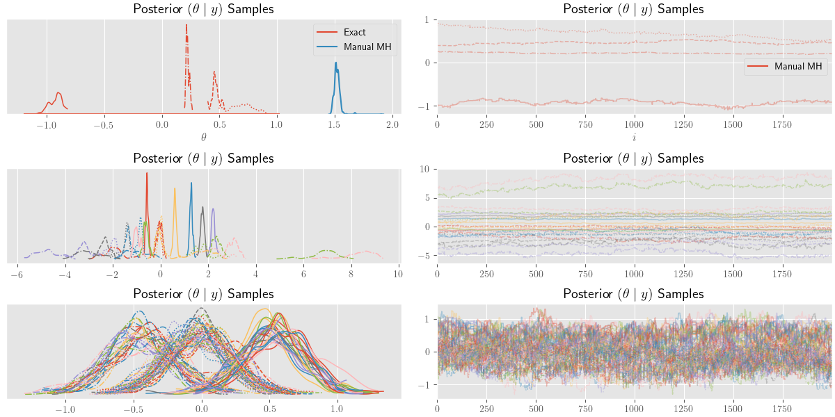
As per the basic examples in the PyMC3 notebooks, the posterior samples are plotted below using the following code:
import matplotlib.pyplot as plt


plt.style.use("ggplot")
plt.rc("text", usetex=True)

tp_axes = pm.traceplot(sample_traces)
We can also superimpose the true posterior density given by \(\eqref{eq:theta-posterior}\) with the following:
import seaborn as sns

import matplotlib.pyplot as plt


plt.style.use("ggplot")
plt.rc("text", usetex=True)

tp_axes = pm.traceplot(sample_traces)

_ = [a_.set_title(r"Posterior $(\theta \mid y)$ Samples") for a_ in tp_axes.ravel()]

freq_axis = tp_axes[0][0]
freq_axis.set_xlabel(r"$\theta$")

sample_axis = tp_axes[0][1]
sample_axis.set_xlabel(r"$i$")

rhs = np.dot(1.0 / tau2, mu) + np.dot(X.T / sigma2, y_obs)
tau_post = 1.0 / tau2 + np.dot(X.T / sigma2, X)

post_mean = rhs / tau_post
post_var_inv = tau_post

post_pdf = partial(scs.norm.pdf, loc=post_mean, scale=1.0 / np.sqrt(post_var_inv))


def add_function_plot(func, ax, num=1e2, label=None):
    post_range = np.linspace(*ax.get_xlim(), num=int(num), endpoint=True)
    post_data = [post_pdf(v) for v in post_range]
    return ax.plot(post_range, post_data, label=label)


# Add true posterior pdf to the plot
add_function_plot(post_pdf, freq_axis, label=r"Exact")

# Add manually produced MH samples to the plot
sns.distplot(theta_samples[:2000], ax=freq_axis, hist=False, label=r"Manual MH")

sample_axis.plot(theta_samples[:2000], label=r"Manual MH")

freq_axis.legend()
sample_axis.legend()
plt.show()
The Costs
MCMC, and specifically the Metropolis-Hastings approach used above, can look very simple and universally applicable, but–of course–there’s a trade-off occurring somewhere. The trade-offs most often appear in relation to the complexity and cost of [intermediate] sampling steps and convergence rates. To over simplify, the standard \(O(N^{-1/2})\) error rate–from the Central Limit Theorem–is the MCMC baseline, which isn’t all that competitive with some of the standard deterministic optimization methods.
Even for conceptually simple models, the proposal distribution (and its parameters) are not always easy to choose or cheap to tune. The upfront computational costs can be quite high for the more generic MCMC approaches, but there are almost always paths toward efficient samplers–in the context of a specific problem, at least.
In practice, the generality and relative simplicity of the Bayes approach, combined with MCMC, can be somewhat misleading to newcomers. After some immediate success with simpler and/or scaled down problems, one is soon led to believe that the cost of direct computations and the effort and skill required to derive efficient methods is not worth the potential parsimony and extra information provided by sample results.
The unfortunate outcome of this situation is sometimes an effective rejection of Bayes and MCMC altogether. Although the point hasn’t been illustrated here, MCMC isn’t the only option. Bayesian models are just as amenable to deterministic estimation as non-Bayesian ones, and a wide array of efficient deterministic estimation techniques are available–albeit not so common in standard practice (Polson, Scott & Willard 2015).
Predictions
The sampling situation offered by MCMC (and Bayes) puts one in a nice situation to make extensive use of predictions and obtain uncertainty measures (e.g. variances, credible intervals, etc.).
In general, posterior predictive samples are fairly easy to obtain. Once you have posterior samples of \(\theta\), say \(\{\theta_i\}_{i=0}^M\), simply plug those into the sampling/observation distribution and sample \(Y\) values. Specifically,
\[\begin{equation} \{y_i \sim p(Y \mid X, \theta_i) : \theta_i \sim p(\theta_i \mid y)\}_{i=0}^M \label{eq:post_predict_samples} \end{equation}\]
is a posterior predictive sample from \(p(Y \mid X, y)\).
The procedural interpretation of \(\eqref{eq:post_predict_samples}\) is:
Assuming we’ve already produced a posterior sample, this is as simple as plugging those \(\theta_i\) into the observation distribution \(\eqref{eq:normal-normal}\) and sampling. The cumulative effect of this process is equivalent to producing an estimate of the marginal
\[ \int p(Y_t \mid x_t, \theta) p(\theta \mid y) d\theta = p(Y_t \mid x_t, y) \;. \]
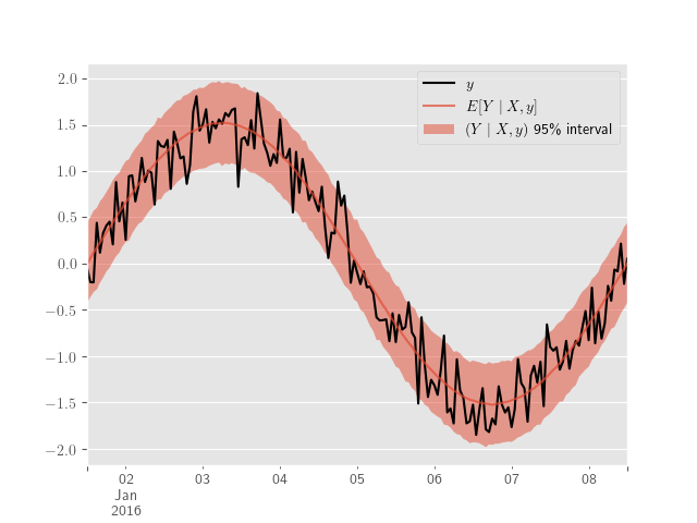
The posterior predictive sample in \(\eqref{eq:post_predict_samples}\) contains much of the information a modeler desires. Take the variance of this sample and one has a common measure of prediction error; produce quantiles of the sample and one has “credible” prediction intervals. The sample produced by mapping an arbitrary function to each posterior predictive sample is itself amenable to the aforementioned summaries, allowing one to easily produce errors for complicated uses of predicted quantities. We illustrate these use cases below.
Using our previous simulation and PyMC3, the posterior predictive samples are obtained with
ppc_samples = pm.sample_posterior_predictive(sample_traces, model=model)and plotted with
y_obs_h = pd.Series(y_obs, index=sim_index)

ppc_hpd = pm.hpd(ppc_samples["Y"], 0.95)

y_obs_h.plot(label="$y$", color="black")

y_obs_mean = pd.Series(ppc_samples["Y"].mean(axis=0), index=sim_index)
y_obs_mean.plot(label=r"$E[Y \mid X, y]$", alpha=0.7)

plt.fill_between(
    sim_index,
    ppc_hpd[:, 0],
    ppc_hpd[:, 1],
    label=r"$(Y \mid X, y)$ 95\% interval",
    alpha=0.5,
)

plt.legend()
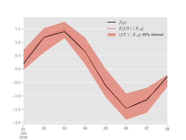
Let’s say we’re interested in daily, monthly, or yearly averages for \(Y_t\) at a lower frequency–like minutes or hours. Similarly, we might want to consider functions of differences between the outputs of different models, \(f(Y^{(j)} - Y^{(k)})\) for \(j, k \in \{1, 2\}\), or more generally \(f(Y^{(j)}, Y^{(k)})\). These quantities derived from simple manipulations of ppc_hpd.
Next, we produce predictions for daily averages–along with (credible) intervals.
ppc_samples_h = pd.DataFrame(ppc_samples["Y"].T, index=sim_index)
ppc_samples_h = ppc_samples_h.stack()
ppc_samples_h = ppc_samples_h[:, 0]

ppc_quantiles_d = ppc_samples_h.resample("D").apply(
    lambda x: x.quantile(q=[0.05, 0.5, 0.95])
)

ppc_quantiles_d = ppc_quantiles_d.unstack()

y_obs_d = y_obs_h.resample("D").mean()
plt.clf()
y_obs_d.plot(label='$f(y)$', color='black')
plt.fill_between(ppc_quantiles_d.index,
ppc_quantiles_d[0.05],
ppc_quantiles_d[0.95],
label=r'$(f(Y) \mid X, y)$ 95\% interval',
alpha=0.5)
ppc_quantiles_d[0.5].plot(label=r'$E[f(Y) \mid X, y]$', alpha=.7)
plt.legend()
plt.show()
Hierarchical Extensions
Even though we only considered “in-sample” predictions in the previous section, out-of-sample and missing values are covered by exactly the same process (neatly simplified by PyMC3’s sample_ppc). In our example we needed an exogenous variable \(x_t\) in order to sample a point from the observation model \((Y_t \mid x_t)\). When the values in \(X\) cannot be obtained–e.g. future values of a non-deterministic quantity–clever, context specific imputations are usually proposed.
Nearly every instance of such imputations gives rise to an implicit model. Going back to our preference for transparent statistical specification, it behooves us to formally specify the model. If we do so in a well-defined Bayes way, then we’re immediately provided the exact same conveniences as above.
If the \(X\) values in our sample now correspond to, say, temperature, and today is the last day in our time-indexed observations y_obs, then predicting forward in time will require temperatures for the future.
One answer to this situation is a model for \(x_t\). If we specify some \(X_t \sim P\), then we can apply the same principles above via the posterior predictive \(p(X_t)\). This posterior predictive will have no exogenous dependencies (unless we want it to), and its posterior can be estimated with our given \(X\) observations. All this occurs in exactly the same fashion as our model for \(Y_t\).
In practice, one often sees the use of summary statistics from previous \(x_t\) observations in intervals representative of the desired prediction period. For instance, in the context of Example 2, the average temperatures in previous years over the months corresponding to the prediction interval (e.g. January-February averages through 2010 to 2016 as imputations for January-February 2017).
This isn’t a bad idea, per se, but it is a needlessly indirect–and often insufficient–approach to defining a statistical model for \(X\). It leaves out critical distributional details, the same details needed to determine how anything using our new \(x_t\) estimates might be affected (through propagation of uncertainty). Eventually one comes around to specifying these details, but, in situations of sufficient complexity, this practice doesn’t produce a very clean, manageable or easily extensible model.
The kinds of complicated models arising in these situations are both conceptually and technically difficult to use, and–as a result–it can be very hard to produce anything other than naive asymptotic approximations for errors and intervals. Sadly, these approximations are generally insufficient for all but the simplest scenarios.
In contrast, we can model the \(x_t\) values directly and have a very clear cut path toward out-of-sample predictions and their distributional properties. Even if we hold to the belief that the previous average values are a reasonable imputation, then a number of simple models can account for that assumption.
Let’s consider a normal regression model for \(x_t\) with seasonal factors, i.e.
\[\begin{equation} X_t \sim \operatorname{N}(d(t)^\top \beta, I \sigma_x^2) \label{eq:exogenous_model} \end{equation}\]
where \(d(t)\) is an indicator vector containing the seasonal factors and \(I\) is an identity matrix.
Keep in mind that we’ve stretched the notation a bit by letting \(X_t\) be a random vector at time \(t\), while \(X\) is still the stacked matrix of observed \(x_t\) values. Now, we’re simply adding the assumption \(x_t \sim X_t\).
Let’s say that our new \(\beta\) vector has terms for each day of the week; this means the matrix of stacked \(d(t)\) values, \(D\), is some classical factor design matrix with levels for each day. The product \(d(t)^\top \beta\) is then some scalar mean for the day corresponding to \(t\).
A simple substitution of this model for our previously constant \(X\) matrix, results in a sort of hierarchical model, which we can now coherently marginalize and obtain the desired posterior predictive, \(p(Y \mid y)\). This time, the posterior predictive is independent of \(X_t\), so we can produce results for any \(t\).
The change in our complete model is relatively minimal. The model above for \(X\) results in the following marginal observation model:
\[\begin{align*} \left(Y_t \mid \beta, \theta \right) &\propto \int p(Y_t \mid X_t, \theta) p(X_t \mid \beta) dX \\ &\sim \operatorname{N}\left( d(t)^\top \beta \cdot \theta, \sigma^2 + \sigma_x^2 \cdot d(t)^\top \beta \beta^\top d(t) \right) \;. \end{align*}\]
The reduction in Example 3 could be considered an entire re-definition of our initial observation model in \(\eqref{eq:normal-normal}\). A change like this is a natural part of the standard model development cycle. However, this is not the only way to look at it. In the Bayesian setting we can keep the observation model fixed and iterate on the prior’s specification. The resulting marginal distribution could effectively be the same under both approaches (if desired), but the latter has the advantage of at least maintaining–conditionally–our earlier work.
We haven’t given a prior to \(\beta\), but if we did, in the absence of conflicting assumptions, we might want the product \(\beta \cdot \theta\) to simplify to a single unknown variables of its own, so that we’re not estimating two “entangled” variables. This idea might be inspired by an understanding of the classical identification issue arising from such products.
With \(\beta\) constant, the form of our marginal observation model is basically unchanged from our initial \(\eqref{eq:normal-normal}\) under \(x_t \to d(t)^\top \beta\) and \(\sigma^2 \to \sigma^2 + \sigma_x^2 \cdot d(t)^\top \beta \beta^\top d(t)\).
Adherence to established models or industry standards is not uncommon. Outside of hierarchical model development, it can be very difficult to make these connections and coherently propagate statistical assumptions.
This model development process expands in complexity and applicability through natural and compartmental extensions of existing terms. Simpler, “base” models are found as marginalizations of the new terms, and all the same estimation techniques apply.
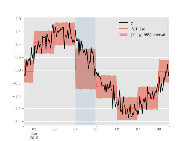
We’ll close with an illustration of the piecewise exogenous variable model described in 6. A few days are added to demonstrate out-of-sample predictions and the design matrix, \(D\), for \(\eqref{eq:exogenous_model}\) is produced using Patsy.
import patsy


ext_sim_index = pd.date_range(
    start="2016-01-01 12:00:00", end="2016-01-16 12:00:00", freq="H"
)

y_obs_df = pd.DataFrame(y_obs, index=sim_index, columns=[r"y"])

# The extra out-of-sample days are set to NaN
# y_obs_df = y_obs_df.reindex(ext_sim_index)

y_obs_df = y_obs_df.assign(weekday=y_obs_df.index.weekday)

y_df, D_df = patsy.dmatrices("y ~ C(weekday)", y_obs_df, return_type="dataframe")

# Create a missing day
y_df.iloc[y_df.index.weekday == 0, 0] = np.nan
Again, with PyMC3 our model and its extension are easily expressed, and the missing observations will be sampled automatically.
import theano.tensor as tt


with pm.Model() as model:
    theta = pm.Normal("theta", mu=mu, tau=1.0 / tau2)
    beta = pm.Normal("beta", mu=0, sd=1e1, shape=(D_df.shape[-1],))
    mu_y = tt.transpose(tt.dot(D_df, beta)) * theta

    Y = pm.Normal("Y", mu=mu_y, tau=1.0 / sigma2, observed=y_df.y)

with model:
    sample_steps = [pm.Metropolis([theta]), pm.Metropolis([beta])]

    if Y.missing_values is not None:
        sample_steps += [pm.Metropolis(Y.missing_values)]

    sample_traces = pm.sample(2000, sample_steps)

    ppc_samples = pm.sample_posterior_predictive(sample_traces)
The posterior predictive results are plotted below.
ppc_y_samples = ppc_samples['Y']

ppc_mean_df = pd.DataFrame(ppc_y_samples.mean(axis=0),
                           index=sim_index,
                           columns=[r'$E[Y \mid y]$'])

ppc_hpd = pd.DataFrame(pm.hpd(ppc_y_samples, 0.95),
                       index=sim_index)

y_obs_df.y.plot(color='black', subplots=False)

missing_ins_range = sim_index[sim_index.weekday == 0]
plt.axvspan(missing_ins_range.min(), missing_ins_range.max(), alpha=0.1)

plt.fill_between(sim_index,
                 ppc_hpd[0].values,
                 ppc_hpd[1].values,
                 label=r'$(Y \mid y)$ 95\% interval',
                 alpha=0.5)

ppc_mean_df.plot(ax=plt.axes(), alpha=0.7)

plt.legend()
Bibliography
Gelman, Carlin, Stern, Dunson, Vehtari & Rubin, Bayesian Data Analysis, CRC Press (2013). ↩︎
Polson, Scott & Willard, Proximal Algorithms in Statistics and Machine Learning, Statistical Science, 30(4), 559–581 (2015). link. ↩︎
Comments
comments powered by Disqus