Introduction
In A Role for Symbolic Computation in the General Estimation of Statistical Models, I described how symbolic computation is used by bayesian modeling software like PyMC3 and some directions it could take. It closed with an example of automatic normal-normal convolution using PyMC3 objects and Theano’s optimization framework. This article elaborates on the foundations for symbolic mathematics in Theano and PyMC3; specifically, its current state, some challenges, and potential improvements.
Let’s start by reconsidering the simple normal-normal convolution model. Mathematically, we can represent the model as follows:
\[\begin{equation} X \sim N(0, 1), \quad Y \sim N\left(1, \frac12\right), \quad Z = X + Y \sim N\left(1, \frac32\right) \label{eq:norm_conv_model} \end{equation}\]
Using PyMC3, the model for Equation \(\eqref{eq:norm_conv_model}\) is constructed as follows:
import sys
import os

from pprint import pprint

import numpy as np

os.environ['MKL_THREADING_LAYER'] = 'GNU'

import theano
import theano.tensor as tt

theano.config.mode = 'FAST_COMPILE'
theano.config.exception_verbosity = 'high'

import pymc3 as pm
mu_X = tt.vector('mu_X')
mu_X.tag.test_value = np.array([0.], dtype=tt.config.floatX)
sd_X = tt.vector('sd_X')
sd_X.tag.test_value = np.array([1.], dtype=tt.config.floatX)
mu_Y = tt.vector('mu_Y')
mu_Y.tag.test_value = np.array([1.], dtype=tt.config.floatX)
sd_Y = tt.vector('sd_Y')
sd_Y.tag.test_value = np.array([0.5], dtype=tt.config.floatX)
with pm.Model() as conv_model:
X_rv = pm.Normal('X_rv', mu_X, sd=sd_X, shape=(1,))
Y_rv = pm.Normal('Y_rv', mu_Y, sd=sd_Y, shape=(1,))
Z_rv = X_rv + Y_rvThe Python objects representing terms in \(\eqref{eq:norm_conv_model}\) are X_rv, Y_rv, and Z_rv in pymc3_model. Those terms together form a Theano graph for the entirety of \(\eqref{eq:norm_conv_model}\).
Other aspects of the model are implicitly stored in the Python context object conv_model. For example, the context object tracks the model’s log likelihood function when some variables are designated as “observed”–i.e. associated with sample data. In this example, we haven’t specified an observed variable, so the context object won’t be immediately useful.
In what follows, we’ll briefly introduce the internal aspects of PyMC3 that are immediately relevant for the topics addressed here; otherwise, see the PyMC3 developer’s guide for an explanation of its design and internal workings.
The terms X_rv, Y_rv are derived from both a PyMC3 Factor class and the standard Theano TensorVariable, as illustrated in the output of pymc3_mro. However, the convolution term Z_rv is not a PyMC3 random variable; in other words, it does not implement the PyMC3 Factor class, but it is a Theano TensorVariable.
pprint({'Y_rv': type(Y_rv).mro()})
pprint({'Z_rv': type(Z_rv).mro()}){'Y_rv': [<class 'pymc3.model.FreeRV'>,
<class 'pymc3.model.Factor'>,
<class 'theano.tensor.var.TensorVariable'>,
<class 'theano.tensor.var._tensor_py_operators'>,
<class 'theano.gof.graph.Variable'>,
<class 'theano.gof.graph.Node'>,
<class 'theano.gof.utils.object2'>,
<class 'object'>]}
{'Z_rv': [<class 'theano.tensor.var.TensorVariable'>,
<class 'theano.tensor.var._tensor_py_operators'>,
<class 'theano.gof.graph.Variable'>,
<class 'theano.gof.graph.Node'>,
<class 'theano.gof.utils.object2'>,
<class 'object'>]}
While PyMC3 doesn’t need to support convolution, so much within Bayesian statistics, MCMC, and probabilistic programming rely on it in some way. It’s an intrinsic part of the algebra(s) implied by the use of probability theory and essential to the implementation of more sophisticated models and sampler optimizations–in at least the same way as symbolic differentiation. Here, the question isn’t whether these algebraic properties are explicitly supported, but how easily they can be implemented when necessary.
As it appears, all work related to probability theory or the algebra of random variables is performed implicitly within the context of Theano and mostly detached from the model-level meta information provided by the PyMC3 abstractions. This means that the linear/tensor algebra supported by Theano is the primary level of abstraction.
More specifically, one purpose of the PyMC3 probability theory abstractions (e.g. random variable classes—FreeRV and ObservedRV, distributions and their likelihoods, etc.) is to associate a PyMC3 Distribution object with a Theano TensorVariable. This connection is made through a distribution attribute
pprint(Y_rv.distribution)
pprint(X_rv.distribution)<pymc3.distributions.continuous.Normal object at 0x7f5d1796e908>
<pymc3.distributions.continuous.Normal object at 0x7f5d17b10208>
Distribution objects loosely represents a measure, holding distribution parameters (e.g. mean and standard deviation mu_X, sd_X) and constructing the appropriate conditional log likelihoods–from which the model’s total log likelihood is later derived. The distribution parameters and log-likelihoods are Theano TensorVariables–including other PyMC3-derived TensorVariables corresponding to (the output of) random variables.
Again, since objects derived via algebraic manipulation of random variables are not themselves random variables within the framework of PyMC3, objects like Z_rv do not have a Distribution attribute. The mechanics described here provide a means for supporting terms like Z_rv with the appropriate “derived” distribution.
To start, we’ll have to dive deeper into the graph aspects of Theano.
Random Variables in Graphs
The Theano graph representing \(\eqref{eq:norm_conv_model}\) consists of linear/tensor algebra operations–under the interface of theano.gof.op.Op–on TensorVariables. For our example in pymc3_model, a textual representation is given in Z_rv_debugprint and a graphical form in fig:norm_sum_graph.
tt.printing.debugprint(Z_rv)Elemwise{add,no_inplace} [id A] ''
|X_rv [id B]
|Y_rv [id C]
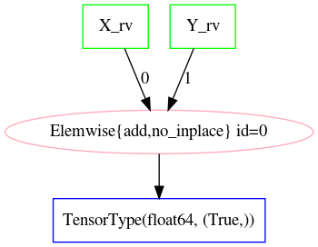
Z_rv for the PyMC3 model in 2.
At present, PyMC3 (version print(pm.__version__) 3.3) does not make very consistent use of Theano’s graph objects. For instance, notice how the dependent parameters mu_X and sd_X are not present in the model’s graph (e.g. fig:norm_sum_graph). We know that X_rv and Y_rv are PyMC3 random variables, but what we see in the graph is only their representations as sampled scalar/vector/matrix/tensor values. In other words, where \(X\), \(Y\) symbolize random variables and \(x \sim X\), \(y \sim Y\) their samples, we have a graph expressing only \(z = x + y\).
What we need for higher-level work is a graph of \(Z = X + Y\) that includes every term involved. This is true for graphs representing a model’s measure/log-likelihood and its sampled values. The former is essentially covered by the log-likelihood graphs we can already produce using the PyMC3 model objects. It’s the latter that we’ll establish here, since it sets the stage for applications of numerous techniques in statistics and probability theory.
One way to produce graphs that represent the full probabilistic model is to formalize the notion of random variables using the Theano API. Basically, if we want to include the relationships between distribution parameters and sampled variables, we need an Op that represents random variables and/or the act of sampling. theano.tensor.raw_random.RandomFunction does exactly this; although it represents the concept of a sampling action and not exactly a random measure.
Nonetheless, using RandomFunction, we can replace nodes corresponding to PyMC3 random variables with newly constructed Op nodes.
We can produce the types of graphs described above through conversion of existing PyMC3 models.
In order to perform any manipulations on our model’s graph, we need to create a Theano theano.gof.FunctionGraph object. We create a utility function in model_graph_fn that constructs a FunctionGraph from a PyMC3 model.
from theano.gof import FunctionGraph, Feature, NodeFinder
from theano.gof.graph import inputs as tt_inputs, clone_get_equiv

def model_graph(pymc_model, derived_vars=None):

    model = pm.modelcontext(pymc_model)

    if derived_vars is not None:
        model_outs = derived_vars
    else:
        model_outs = [o.logpt for o in model.observed_RVs]

    model_inputs = [inp for inp in tt_inputs(model_outs)]
    # if not isinstance(inp, theano.gof.graph.Constant)]

    model_memo = clone_get_equiv(model_inputs, model_outs,
                                 copy_orphans=False)

    fg_features = [
        NodeFinder(),
    ]
    model_fg = FunctionGraph([model_memo[i] for i in model_inputs],
                             [model_memo[i] for i in model_outs],
                             clone=False, features=fg_features)
    model_fg.memo = model_memo

    return model_fg
When cloning the graph with theano.gof.graph.clone_get_equiv in model_graph, we lose the FreeRV.distribution attribute–among others. Since those attributes hold all the information required to construct our RandomFunction Ops, we’ll need to find a way to preserve it.
This can be accomplished by overriding the default Theano clone function inherited by the PyMC3 random variable classes.
import types
from copy import copy

pymc_rv_types = (pm.model.FreeRV, pm.model.ObservedRV, pm.model.TransformedRV)

pymc_rv_attrs = ['dshape', 'dsize', 'distribution', 'logp_elemwiset',
                 'logp_sum_unscaledt', 'logp_nojac_unscaledt', 'total_size',
                 'scaling', 'missing_values']

for rv_type in pymc_rv_types:

    if not hasattr(rv_type, '__clone'):
        rv_type.__clone = rv_type.clone

    def pymc_rv_clone(self):
        cp = rv_type.__clone(self)
        for attr in pymc_rv_attrs:
            setattr(cp, attr, copy(getattr(self, attr, None)))

        # Allow a cloned rv to inherit the context's model?
        # try:
        #     cp.model = pm.Model.get_context()
        # except TypeError:
        #     pass

        if getattr(cp, 'model', None) is None:
            cp.model = getattr(self, 'model', None)

        return cp

    rv_type.clone = pymc_rv_clone
Now, we can produce a proper FunctionGraph from our PyMC3 model.
Z_fgraph_tt = model_graph(conv_model, derived_vars=[Z_rv])With a FunctionGraph at our disposal, we can use the graph manipulation tools provided by Theano to replace the PyMC3 TensorVariables used to represent random variables with corresponding Theano RandomFunctions that represent the act of sampling to produce said random variables.
We can use a simple mapping between Pymc3 random variable nodes and RandomFunction to specify the desired replacements. Fortunately, this isn’t too difficult, since RandomFunction already supports numerous Numpy-provided random distributions–covering much of the same ground as the PyMC3 distributions. Otherwise, the rest of the work involves mapping distribution parameters.
Also, RandomFunction requires a RandomStream, which it uses to track the sampler state. For our purely symbolic purposes, the stream object is not immediately useful, but it does–in the end–provide a sample-able graph as a nice side-effect. We demonstrate the PyMC3 random variable-to-RandomFunction translation in random_op_mapping using only a single mapping.
from theano.tensor.raw_random import RandomFunction

pymc_theano_rv_equivs = {
    pm.Normal:
    lambda dist, rand_state:
    tt.raw_random.normal(rand_state, dist.shape.tolist(), dist.mu, dist.sd),
}
def create_theano_rvs(fgraph, clone=True, rand_state=None):
"""Replace PyMC3 random variables with `RandomFunction` Ops.
TODO: Could use a Theano graph `Feature` to trace--or even
replace--random variables.
Parameters
----------
fgraph : FunctionGraph
A graph containing PyMC3 random variables.
clone: bool, optional
Clone the original graph.
rand_state : RandomStateType, optional
The Theano random state.
Returns
-------
out : A cloned graph with random variables replaced and a `memo` attribute.
"""
if clone:
fgraph_, fgraph_memo_ = fgraph.clone_get_equiv(attach_feature=False)
fgraph_.memo = fgraph_memo_
else:
fgraph_ = fgraph
if rand_state is None:
rand_state = theano.shared(np.random.RandomState())
fgraph_replacements = {}
fgraph_new_inputs = set()
for old_rv_i, old_rv in enumerate(fgraph_.inputs):
if isinstance(old_rv, pymc_rv_types):
dist = old_rv.distribution
theano_rv_op = pymc_theano_rv_equivs.get(type(dist), None)
if theano_rv_op is not None:
rng_tt, new_rv = theano_rv_op(dist, rand_state)
# Keep track of our replacements
fgraph_replacements[old_rv] = new_rv
new_rv.name = '~{}'.format(old_rv.name)
new_rv_inputs = [i for i in tt_inputs([new_rv])]
fgraph_new_inputs.update(new_rv_inputs)
else:
print('{} could not be mapped to a random function'.format(old_rv))
fgraph_new_inputs_memo = theano.gof.graph.clone_get_equiv(
fgraph_new_inputs, list(fgraph_replacements.values()),
copy_orphans=False)
# Update our maps and new inputs to use the cloned objects
fgraph_replacements = {old_rv: fgraph_new_inputs_memo.pop(new_rv)
for old_rv, new_rv in fgraph_replacements.items()}
fgraph_new_inputs = set(map(fgraph_new_inputs_memo.pop, fgraph_new_inputs))
# What remains in `fgraph_new_inputs_memo` are the nodes between our desired
# inputs (i.e. the random variables' distribution parameters) and the old inputs
# (i.e. Theano `Variable`s corresponding to a sample of said random variables).
_ = [fgraph_.add_input(new_in) for new_in in fgraph_new_inputs
if not isinstance(new_in, theano.gof.graph.Constant)]
# _ = [fgraph_.add_input(new_in) for new_in in fgraph_new_inputs_memo.values()]
fgraph_.replace_all(fgraph_replacements.items())
# The replace method apparently doesn't remove the old inputs...
_ = [fgraph_.inputs.remove(old_rv) for old_rv in fgraph_replacements.keys()]
return fgraph_Z_fgraph_rv_tt = create_theano_rvs(Z_fgraph_tt)
tt.printing.debugprint(Z_fgraph_rv_tt)Elemwise{add,no_inplace} [id A] '' 10
|RandomFunction{normal}.1 [id B] '~X_rv' 9
| |<RandomStateType> [id C]
| |Elemwise{Cast{int64}} [id D] '' 8
| | |MakeVector{dtype='int8'} [id E] '' 7
| | |TensorConstant{1} [id F]
| |mu_X [id G]
| |Elemwise{mul,no_inplace} [id H] '' 6
| |InplaceDimShuffle{x} [id I] '' 5
| | |TensorConstant{1.0} [id J]
| |sd_X [id K]
|RandomFunction{normal}.1 [id L] '~Y_rv' 4
|<RandomStateType> [id C]
|Elemwise{Cast{int64}} [id M] '' 3
| |MakeVector{dtype='int8'} [id N] '' 2
| |TensorConstant{1} [id F]
|mu_Y [id O]
|Elemwise{mul,no_inplace} [id P] '' 1
|InplaceDimShuffle{x} [id Q] '' 0
| |TensorConstant{1.0} [id J]
|sd_Y [id R]
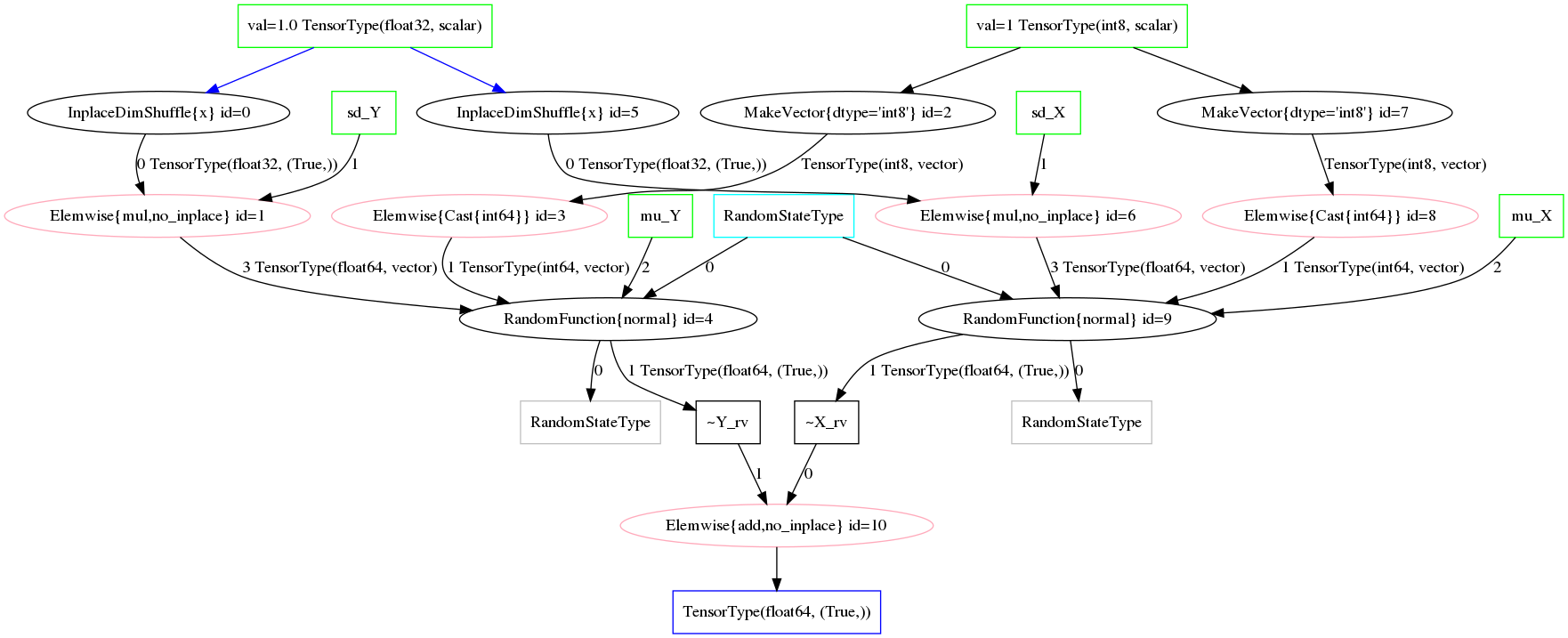
Op to represent sampling/a random variable.
Illustrations of the transformed graphs given in random_op_mapping_exa and fig:random_op_mapping_exa_graph show the full extent of our simple example model and provide a context in which to perform higher-level manipulations.
With a graph representing the relevant terms and relationships, we can implement the convolution simplification/transformation/optimization. For instance, as shown in rv_find_nodes, we can now easily query random function/variable nodes in a graph.
# Using a `FunctionGraph` "feature"
Z_fgraph_rv_tt.attach_feature(NodeFinder())

# The fixed `TensorType` is unnecessarily restrictive.
rf_normal_type = RandomFunction('normal', tt.TensorType('float64', (True,)))
rf_nodes = Z_fgraph_rv_tt.get_nodes(rf_normal_type)

#
# or, more generally,...
#
def get_random_nodes(fgraph):
    return list(filter(lambda x: isinstance(x.op, RandomFunction), fgraph.apply_nodes))

rf_nodes = get_random_nodes(Z_fgraph_rv_tt)

tt.printing.debugprint(rf_nodes)
RandomFunction{normal}.0 [id A] ''
|<RandomStateType> [id B]
|Elemwise{Cast{int64}} [id C] ''
| |MakeVector{dtype='int8'} [id D] ''
| |TensorConstant{1} [id E]
|mu_X [id F]
|Elemwise{mul,no_inplace} [id G] ''
|InplaceDimShuffle{x} [id H] ''
| |TensorConstant{1.0} [id I]
|sd_X [id J]
RandomFunction{normal}.1 [id A] '~X_rv'
RandomFunction{normal}.0 [id K] ''
|<RandomStateType> [id B]
|Elemwise{Cast{int64}} [id L] ''
| |MakeVector{dtype='int8'} [id M] ''
| |TensorConstant{1} [id E]
|mu_Y [id N]
|Elemwise{mul,no_inplace} [id O] ''
|InplaceDimShuffle{x} [id P] ''
| |TensorConstant{1.0} [id I]
|sd_Y [id Q]
RandomFunction{normal}.1 [id K] '~Y_rv'
Performing High-level Simplifications
To apply optimizations like our simple convolution, we need to first identify the appropriate circumstances for its application. This means finding all sub-graphs for which we are able to replace existing nodes with a convolution node.
Theano provides some unification tools that facilitate the search component. We’ll use those to implement an extremely restrictive form of our convolution.
In normal_conv_pattern, we create patterns for our expressions of interest that are unified against the elements in our graph and reified with a replacement expression. The patterns are expressed as tuples in a LISP-like fashion, e.g. (add, 1, 2) corresponding to an unevaluated add(1, 2).
from operator import attrgetter, itemgetter


# FIXME: This fixed `TensorType` specification is restrictive.
NormalRV = RandomFunction('normal', tt.TensorType('float64', (True,)))

norm_conv_pat_tt = [
    tt.gof.opt.PatternSub(
        # Search expression pattern
      (tt.add,
       (NormalRV, 'rs_x', 'shp_x', 'mu_x', 'sd_x'),
       (NormalRV, 'rs_y', 'shp_y', 'mu_y', 'sd_y'),
      ),
        # Replacement expression
      (itemgetter(1), #
       (NormalRV,
        'rs_x',
        'shp_x',
        (tt.add, 'mu_x', 'mu_y'),
        (tt.sqrt, (tt.add, (tt.square, 'sd_x'), (tt.square, 'sd_y'))),
       )),
    ),
]
The itemgetter(1) applied to the replacement result is necessary because the Op RandomFunction returns two outputs and the second is the TensorVariable corresponding to a sample from that random variable.
We also need to specify exactly how the pattern matching and replacement are to be performed for the entire graph. Do we match a single sum of normal distributions or all of them? What happens when a replacement creates yet another sum of normals that can be reduced?
In this case, we choose to apply the operation until it reaches a fixed point, i.e. until it produces no changes in the graph.
norm_conv_opt_tt = tt.gof.opt.EquilibriumOptimizer(norm_conv_pat_tt,
                                                   max_use_ratio=10)
Finally, we manually perform our Theano optimization.
_ = norm_conv_opt_tt.optimize(Z_fgraph_rv_tt)The optimization was applied within our graph, as evidenced by the single new RandomFunction node.
tt.printing.debugprint(Z_fgraph_rv_tt)RandomFunction{normal}.1 [id A] '' 11
|<RandomStateType> [id B]
|Elemwise{Cast{int64}} [id C] '' 10
| |MakeVector{dtype='int8'} [id D] '' 9
| |TensorConstant{1} [id E]
|Elemwise{add,no_inplace} [id F] '' 8
| |mu_X [id G]
| |mu_Y [id H]
|Elemwise{sqrt,no_inplace} [id I] '' 7
|Elemwise{add,no_inplace} [id J] '' 6
|Elemwise{sqr,no_inplace} [id K] '' 5
| |Elemwise{mul,no_inplace} [id L] '' 4
| |InplaceDimShuffle{x} [id M] '' 3
| | |TensorConstant{1.0} [id N]
| |sd_X [id O]
|Elemwise{sqr,no_inplace} [id P] '' 2
|Elemwise{mul,no_inplace} [id Q] '' 1
|InplaceDimShuffle{x} [id R] '' 0
| |TensorConstant{1.0} [id N]
|sd_Y [id S]
Likewise, the resulting distribution terms in the optimized graph reflect the normal-normal random variable sum. Figure fig:norm_sum_merge_graph shows the graph under our optimization.
conv_rv_tt = Z_fgraph_rv_tt.outputs[0].owner

new_mu, new_sd = conv_rv_tt.inputs[2:4]

# Test values of the original means/new moments' inputs
print(', '.join(['{} = {}'.format(tt.pprint(o), o.tag.test_value)
                 for o in new_mu.owner.inputs]))
print(tt.pprint(new_mu))

print(', '.join(['{} = {}'.format(tt.pprint(o), o.tag.test_value)
                 for o in new_sd.owner.inputs]))
print(tt.pprint(new_sd))

print('mean: {}\nstd. dev.: {}'.format(
    new_mu.tag.test_value,
    new_sd.tag.test_value))
mu_X = [0.], mu_Y = [1.]
(mu_X + mu_Y)
(sqr((TensorConstant{1.0} * sd_X)) + sqr((TensorConstant{1.0} * sd_Y))) = [1.25]
sqrt((sqr((TensorConstant{1.0} * sd_X)) + sqr((TensorConstant{1.0} * sd_Y))))
mean: [1.]
std. dev.: [1.11803399]
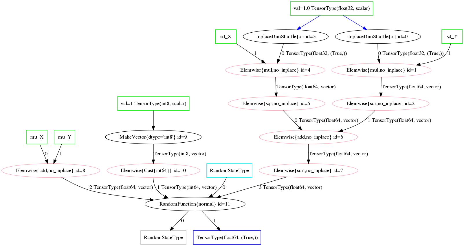
Generalizing Operations
Our example above was admittedly too simple; for instance, what about scale and location transformed variables? Most models/graphs will consist of more elaborate manipulations of random variables, so it’s necessary that we account for as many basic manipulations, as well.
We start by adding an optimization that lifts scale parameters into the arguments/parameters of a random variable. In other words,
\[\begin{gather*} X \sim N(\mu, \sigma^2) \\ Z = a X \sim N\left(a \mu, (a \sigma)^2\right) \;. \end{gather*}\]
norm_conv_pat_tt += [
    tt.gof.opt.PatternSub(
        # Search expression pattern
        (tt.mul,
         'a_x',
         (NormalRV, 'rs_x', 'shp_x', 'mu_x', 'sd_x')),
        # Replacement expression
        (itemgetter(1),
         (NormalRV,
          # RNG
                'rs_x',
          # Convolution shape
                'shp_x',
          # Convolution mean
                (tt.mul, 'a_x', 'mu_x'),
          # Convolution std. dev.
                (tt.mul, 'a_x', 'sd_x'),
         )),
    )
]

norm_conv_opt_tt = tt.gof.opt.EquilibriumOptimizer(
    norm_conv_pat_tt, max_use_ratio=10)
The additional optimization is demonstrated in mat_mul_scaling_exa.
mu_X = tt.vector('mu_X')
mu_X.tag.test_value = np.array([0.], dtype=tt.config.floatX)
sd_X = tt.vector('sd_X')
sd_X.tag.test_value = np.array([1.], dtype=tt.config.floatX)

with pm.Model() as conv_scale_model:
    X_rv = pm.Normal('X_rv', mu_X, sd=sd_X, shape=(1,))
    Z_rv = 5 * X_rv

Z_mul_tt = model_graph(conv_scale_model, derived_vars=[Z_rv])
Z_mul_rv = create_theano_rvs(Z_mul_tt)

Z_mul_rv_merged = Z_mul_rv.clone()

_ = norm_conv_opt_tt.optimize(Z_mul_rv_merged)
fig:scaled_random_sum_before and fig:scaled_random_sum_after demonstrate the a scaled normal random variable before and after the optimization, respectively.
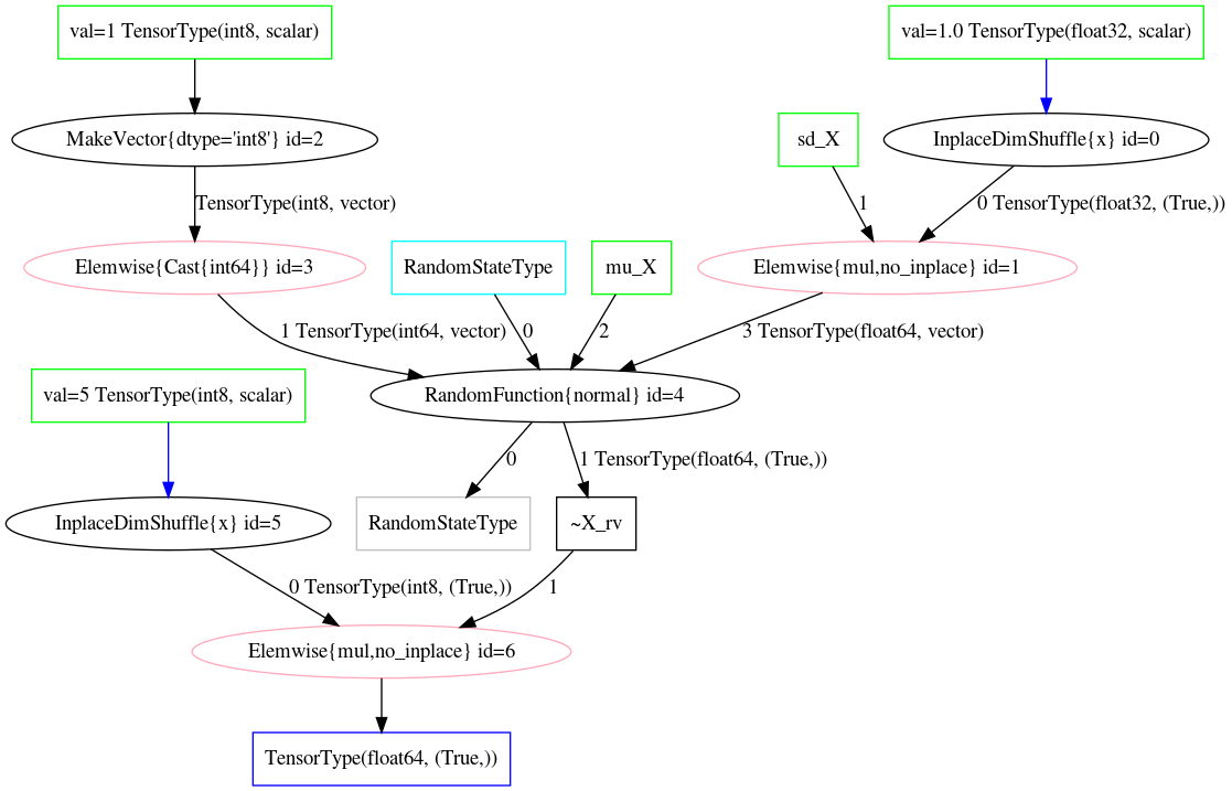
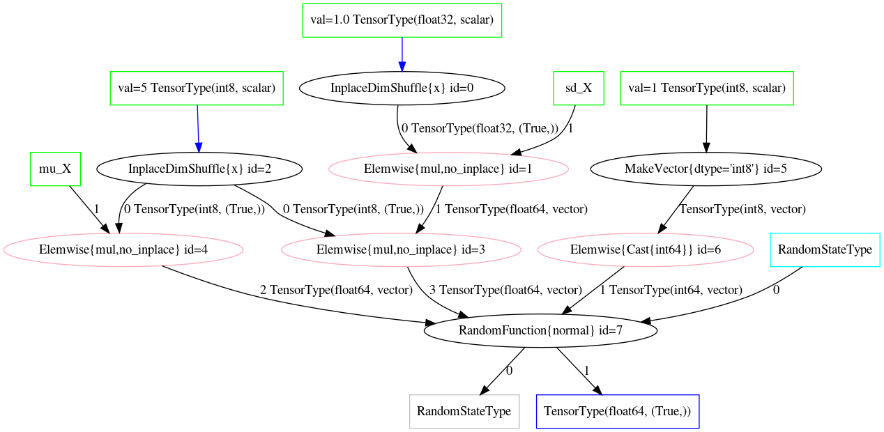
Challenges
If we change the dimensions of our example above, the pattern employed by our scaling optimization will not match. To fix this, we can generalize the form of our RandomFunction operator so that it includes more cases of broadcastable dimensions–instead of only (True, )
We could also extend the reach of our PatternSubs; however, this direction introduces more complexity into the process of writing optimizations and provides no foreseeable benefit elsewhere.
More generally, one of the major challenges in this kind of work is due to the design of RandomFunction; its type is dependent on a TensorType parameter that requires an array of “broadcast” dimensions.
This situation arises–in part–from PyMC3, Theano, and NumPy’s use of a “size” parameter in combination with random variable dimensions inferred from distribution parameters. A few outstanding PyMC3 issues seem to revolve around the interactions between these elements.
The size parameter is like a sample size, but with all the samples considered together as a single tensor (e.g. each sample of a multivariate normal random variable, say, acting as a column in a matrix). The size parameter is independent of a random variable’s parameters’ sizes (e.g. dimensions of a mean and covariance), but, together, the size and distribution parameters effectively compose the size/dimension of a random variable’s support (e.g. the matrix in the above example is the resulting random variable).
Needless to say, PyMC3 and Theano’s terms–and their relation to mathematical notions–are a bit confusing, and likely driven more by software design choices than the mathematical frameworks in use. However, those design choices significantly affect our ability to manipulate graphs and express common mathematical notions. For instance, these terms and design choices put greater demand on the graph manipulation steps, due to the ambiguous dimensions of the elements involved.
Next Steps
In a follow-up, I’ll introduce a new Op that overcomes some of the dimensionality issues and allows for much easier graph manipulation. It replaces RandomFunction with a single Op for each distribution type and [re]moves the type specifier from the definition of the Op.
Essentially, the TensorType argument to the RandomFunction constructor is moved into RandomFunction’s make_node method and, thus, generated/inferred from the symbolic inputs.
To be clear, we’re talking about two distinct aspects of RandomFunction: one is the NormalRV = RandomFunction('normal', TensorType('float64', bcast)) step, in which we create the Op corresponding to a specific type of normal random variable, and the other in which we use the Op (e.g. NormalRV(rng, 1, 2))–to, say, produce a tensor variable corresponding to an instance of said random variable.
This distinction is important for pattern matching because NormalRV, as defined above, isn’t very general and mostly due to the TensorType('float64', bcast)) covering only some Theano tensor types (i.e. those that match the fixed broadcast dimensions specified by bcast).
As stated previously, there have been real difficulties with the handling of shape and type information in PyMC3 (see PyMC3 PR 1125). These problems are related to the same concerns involving TensorTypes. In refactoring the type information requirement for RandomFunction, we’ll end up addressing those PyMC3 issues as well.
Bibliography
[WillardRoleSymbolicComputation2017] Willard, A Role for Symbolic Computation in the General Estimation of Statistical Models, Brandon T. Willard, (2017). link. ↩︎
Comments
comments powered by Disqus